15 Introdction to First-Order Differential Equations
15.1 Modeling Change
Throughout calculus, we have studied functions f : \mathbb{R} \to \mathbb{R} and their derivatives f'(x). The derivative encodes the instantaneous rate of change—given the current state x, it tells us how rapidly f is changing. We developed techniques to compute derivatives of known functions and used them to analyze behavior: extrema, concavity, approximation.
But many natural processes reverse this direction. We don’t start with a function and compute its rate of change. Instead, we observe rates of change and seek to reconstruct the underlying function. A physicist measures velocity and wants position. A biologist observes population growth rates and wants population size. An engineer specifies how a system responds to inputs and wants the system’s state over time.
These problems take the form: given information about f', find f.
When the relationship is simple—f'(x) = g(x) for some known g—integration solves the problem: f(x) = \int g(x) \, dx. But often, the rate of change depends on the current state itself: the growth rate of a population depends on the current population size, the velocity of a falling object depends on its current position, the temperature change in a cooling object depends on its current temperature.
This leads to equations of the form \frac{dy}{dx} = F(x, y), where the derivative dy/dx is specified as a function of both the independent variable x and the unknown function y(x) itself. Such equations are differential equations—equations involving derivatives, not just algebraic expressions.
A solution is a function y(x) that satisfies the equation identically on some interval. Finding solutions means reconstructing the function from knowledge of how it changes.
15.2 Direction Fields and Geometry
Consider the differential equation \frac{dy}{dx} = y.
This says: at any point (x, y), the slope of the solution curve passing through that point equals y. We don’t yet know the solution, but we know the local behavior everywhere.
At (0, 1): slope = 1. The solution curve passing through this point must have tangent line y = 1 + x locally.
At (0, 2): slope = 2. The tangent line is y = 2 + 2x.
At (0, -1): slope = -1. The tangent line is y = -1 - x.
At each point in the plane, the differential equation specifies a direction—the slope of any solution curve passing through that point. We can visualize this by drawing small line segments with the appropriate slopes at many points.
The direction field shows the flow of solutions. Solution curves follow the field lines like particles in a fluid. This geometric perspective—viewing differential equations as defining vector fields on the plane—connects to differential geometry: solutions are integral curves of the vector field (1, F(x,y)).
Each integral curve is tangent to the direction field at every point along it. Different initial conditions produce different curves, but they all respect the same local direction constraints.
This visualization reveals structure before solving anything algebraically. We see that solutions spread apart exponentially, that there’s a unique curve through each point, and that curves never cross (since two curves crossing would mean two different slopes at the same point, contradicting a later result Theorem 15.1).
15.3 Initial Value Problems
A differential equation alone does not determine a unique solution. For \frac{dy}{dx} = y, any function y = Ce^x satisfies the equation for any constant C. The equation specifies how solutions change but not where they start.
To specify a unique solution, we impose an initial condition: we require the solution to pass through a particular point (x_0, y_0).
Definition 15.1 (Initial Value Problem) An initial value problem (IVP) consists of: \frac{dy}{dx} = F(x, y), \quad y(x_0) = y_0.
A solution is a function y(x) satisfying both the differential equation and the initial condition.
Example 15.1 (Initial Value Problem) Solve \frac{dy}{dx} = y with y(0) = 3.
We know the general solution is y = Ce^x. Imposing y(0) = 3 gives C = 3, so y(x) = 3e^x.
This is the unique solution passing through (0, 3).
The initial value problem pins down one integral curve from the family of all solutions. Geometrically: the direction field defines infinitely many flow lines, and the initial condition selects one.
15.4 Existence and Uniqueness
Does every IVP have a solution? Is that solution unique?
For general F(x,y), these are nontrivial questions. Consider \frac{dy}{dx} = \frac{1}{y}, \quad y(0) = 0.
The direction field is undefined at y = 0 (division by zero). No solution can pass through (0, 0) because we cannot assign a slope there. The IVP has no solution.
Conversely, consider \frac{dy}{dx} = \sqrt{|y|}, \quad y(0) = 0.
Both y(x) = 0 and y(x) = \frac{x^2}{4} for x \geq 0 satisfy the equation and initial condition. Uniqueness fails.
These pathologies occur when F(x,y) is not well-behaved. The fundamental result:
Theorem 15.1 (Existence and Uniqueness (Picard-Lindelöf)) Let F(x,y) be continuous in a rectangle R = \{(x,y) : |x - x_0| \leq a, |y - y_0| \leq b\} and satisfy a Lipschitz condition (stronger form of continuity) in y |F(x, y_1) - F(x, y_2)| \leq L|y_1 - y_2| for all (x, y_1), (x, y_2) \in R and some constant L > 0.
Then the IVP \frac{dy}{dx} = F(x,y), y(x_0) = y_0 has a unique solution on some interval |x - x_0| < h.
Continuity ensures the direction field is defined everywhere. The Lipschitz condition controls how rapidly directions change—it prevents the field from “twisting too sharply.” Together, these ensure that integral curves exist and don’t cross.
The Lipschitz condition is satisfied when \frac{\partial F}{\partial y} is bounded (by the Mean Value Theorem). Most smooth functions satisfy this locally.
Example 15.2 (Lipschitz Condition for Linear Growth) For \frac{dy}{dx} = y, we have F(x,y) = y. Then |F(x, y_1) - F(x, y_2)| = |y_1 - y_2|.
The Lipschitz constant is L = 1. The theorem guarantees unique solutions through every point.
Example 15.3 (Failure of Lipschitz Condition) For \frac{dy}{dx} = \sqrt{|y|}, we have |F(x, y_1) - F(x, y_2)| = |\sqrt{|y_1|} - \sqrt{|y_2|}|.
Near y = 0, this does not satisfy a Lipschitz condition (the derivative \frac{\partial}{\partial y}\sqrt{|y|} = \frac{1}{2\sqrt{|y|}} blows up). Uniqueness fails at (x_0, 0).
15.5 Separation of Variables
The simplest class of solvable first-order equations has the form \frac{dy}{dx} = g(x) h(y), where the right side factors into a function of x alone and a function of y alone. These are separable equations.
Method: Rewrite as \frac{1}{h(y)} \, dy = g(x) \, dx.
Integrate both sides \int \frac{1}{h(y)} \, dy = \int g(x) \, dx + C.
This gives an implicit solution. Solve for y if possible.
Justification: Formally, we’re using the chain rule in reverse. If y = y(x), then \frac{dy}{dx} = g(x) h(y) \implies \frac{1}{h(y)} \frac{dy}{dx} = g(x).
Integrate with respect to x \int \frac{1}{h(y(x))} \frac{dy}{dx} \, dx = \int g(x) \, dx.
The left side is \int \frac{1}{h(y)} \, dy by substitution (u = y(x), du = y'(x) dx).
Example 15.4 (Separation with Quadratic Growth) Solve \frac{dy}{dx} = xy.
Separate: \frac{1}{y} dy = x \, dx. Integrate: \ln|y| = \frac{x^2}{2} + C.
Exponentiate, |y| = e^{x^2/2 + C} = Ae^{x^2/2} where A = e^C > 0. Including both signs y = Ce^{x^2/2}, where C can be any nonzero constant. Note y = 0 is also a solution (the equilibrium solution).
Example 15.5 (Separation Yielding a Circle) Solve \frac{dy}{dx} = -\frac{x}{y} with y(0) = 1.
Separate: y \, dy = -x \, dx. Integrate: \frac{y^2}{2} = -\frac{x^2}{2} + C.
Impose y(0) = 1: \frac{1}{2} = C, so \frac{y^2}{2} = -\frac{x^2}{2} + \frac{1}{2} \implies x^2 + y^2 = 1.
The solution is the upper semicircle y = \sqrt{1 - x^2} for |x| \leq 1.
This illustrates a subtlety: the solution exists only on a finite interval [-1, 1]. Beyond this, y becomes complex. Existence theorems guarantee local solutions but not necessarily global ones.
15.6 The Logistic Equation
In Calculus 1, we introduced the discrete logistic map: P_{n+1} = r P_n \left(1 - \frac{P_n}{K}\right).
This modeled population growth with carrying capacity K. The continuous analogue replaces discrete steps with a differential equation.
Definition 15.2 (Logistic Equation) \frac{dP}{dt} = r P \left(1 - \frac{P}{K}\right).
Here P(t) is population at time t, r > 0 is the intrinsic growth rate, and K > 0 is the carrying capacity.
When P \ll K, the factor (1 - P/K) \approx 1, so \frac{dP}{dt} \approx rP—exponential growth. As P approaches K, the growth rate slows. At P = K, \frac{dP}{dt} = 0—the population stabilizes.
Setting \frac{dP}{dt} = 0 gives P = 0 or P = K. These are equilibrium solutions—constant functions satisfying the equation.
Solution. Rewrite as \frac{1}{P(1 - P/K)} \, dP = r \, dt.
Use partial fractions on the left side. Write \frac{1}{P(1 - P/K)} = \frac{1}{P} + \frac{1/K}{1 - P/K} = \frac{1}{P} + \frac{1}{K - P}.
Integrate \ln|P| - \ln|K - P| = rt + C.
Simplify \ln\left|\frac{P}{K-P}\right| = rt + C.
Exponentiate \frac{P}{K-P} = Ae^{rt}, \quad A = \pm e^C.
Solve for P P = \frac{AKe^{rt}}{1 + Ae^{rt}}.
Impose initial condition P(0) = P_0 P_0 = \frac{AK}{1 + A} \implies A = \frac{P_0}{K - P_0}.
Substitute back P(t) = \frac{K P_0 e^{rt}}{K - P_0 + P_0 e^{rt}} = \frac{K}{1 + \left(\frac{K - P_0}{P_0}\right)e^{-rt}}.
Behavior:
As t \to \infty, e^{-rt} \to 0, so P(t) \to K regardless of P_0 (assuming 0 < P_0 < K).
The population asymptotically approaches the carrying capacity.
Growth is fastest near P = K/2 (inflection point of the logistic curve).
The logistic equation appears throughout biology, ecology, epidemiology, and economics. It models any process with self-limiting growth.
15.7 Euler’s Method
Not all differential equations admit closed-form solutions. When separation of variables fails—or when F(x,y) is too complicated to integrate—we turn to numerical methods.
Euler’s method is the simplest: approximate the solution by following the direction field in small steps.
Definition 15.3 (Euler’s Method) Given \frac{dy}{dx} = F(x,y) with y(x_0) = y_0, partition [x_0, x_N] into n steps of size h = \frac{x_N - x_0}{n}. Define x_{k+1} = x_k + h, \quad y_{k+1} = y_k + h F(x_k, y_k), \quad k = 0, 1, \ldots, n-1.
The sequence (x_k, y_k) approximates the solution curve.
Geometric interpretation: At (x_k, y_k), the slope is F(x_k, y_k). Move along this tangent line a distance h to reach (x_{k+1}, y_{k+1}). Repeat.
This is a discrete approximation to the continuous flow. As h \to 0, the approximation improves.
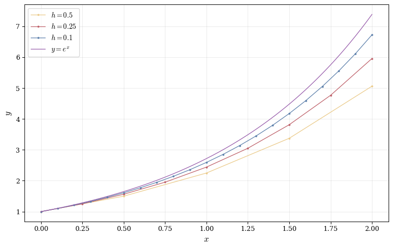
Example 15.6 (Euler’s Method for Exponential Growth) Approximate \frac{dy}{dx} = y, y(0) = 1 on [0, 1] with h = 0.1.
We have F(x,y) = y, x_0 = 0, y_0 = 1. The recursion is y_{k+1} = y_k + 0.1 \cdot y_k = 1.1 y_k.
Thus: \begin{align*} y_0 &= 1 \\ y_1 &= 1.1 \\ y_2 &= 1.21 \\ y_3 &= 1.331 \\ &\vdots \\ y_{10} &= 1.1^{10} \approx 2.594. \end{align*}
The exact solution is y(1) = e \approx 2.718. Euler’s method underestimates (the true solution curves upward more sharply).
As h decreases, the approximation converges to the true solution. The error decreases linearly with h (first-order method).
More sophisticated methods—Runge-Kutta, Adams-Bashforth—achieve higher-order convergence by using derivative information at multiple points. But Euler’s method captures the essential idea: discretize the differential equation and step forward along the direction field.
15.8 Qualitative Analysis: Phase Portraits
Even when we cannot solve a differential equation analytically or numerically, we can extract qualitative behavior from the equation itself. This qualitative theory reveals structure without explicit solutions.
Equilibria: Points where \frac{dy}{dx} = 0. These are constant solutions.
Stability: Does the system return to equilibrium after small perturbations?
- Stable: nearby solutions approach the equilibrium as t \to \infty.
- Unstable: nearby solutions diverge.
- Semi-stable: stable from one side, unstable from the other.
Example 15.7 (Logistic Equation Stability Analysis) \frac{dP}{dt} = rP\left(1 - \frac{P}{K}\right).
Equilibria is at P = 0 and P = K.
Stability analysis:
Linearize near equilibrium. Let P = P^* + \varepsilon where P^* is an equilibrium and \varepsilon is small. Expand: \frac{d\varepsilon}{dt} = r(P^* + \varepsilon)\left(1 - \frac{P^* + \varepsilon}{K}\right) \sim r\left(1 - \frac{2P^*}{K}\right)\varepsilon.
The coefficient \lambda = r\left(1 - \frac{2P^*}{K}\right) determines stability
\lambda < 0: stable (perturbations decay).
\lambda > 0: unstable (perturbations grow).
At P^* = 0: \lambda = r > 0 (unstable).
At P^* = K: \lambda = -r < 0 (stable).
Thus, populations near zero grow away from zero (exponentially at first). Populations near K decay back to K.
This explains the long-term behavior without solving the equation: regardless of initial condition (assuming 0 < P_0 < K), the population approaches the carrying capacity.
15.9 Predator-Prey Systems
Most natural processes involve multiple interacting quantities. Predator-prey dynamics provide a classic example.
Let x(t) = prey population, y(t) = predator population. The Lotka-Volterra equations: \begin{cases} \frac{dx}{dt} = \alpha x - \beta xy \\ \frac{dy}{dt} = \delta xy - \gamma y \end{cases}
Interpretation:
\alpha x: prey reproduce exponentially without predators.
-\beta xy: prey are consumed at a rate proportional to encounters (product of populations).
\delta xy: predators gain energy from prey consumption.
-\gamma y: predators die without prey.
All parameters \alpha, \beta, \delta, \gamma > 0.
Equilibria:
Setting both derivatives to zero x(\alpha - \beta y) = 0, \quad y(\delta x - \gamma) = 0.
Solutions: (0, 0) (extinction) and \left(\frac{\gamma}{\delta}, \frac{\alpha}{\beta}\right) (coexistence).
Nullclines: Curves where one derivative vanishes.
- \frac{dx}{dt} = 0: y = \frac{\alpha}{\beta} (horizontal line) or x = 0 (vertical axis).
- \frac{dy}{dt} = 0: x = \frac{\gamma}{\delta} (vertical line) or y = 0 (horizontal axis).
The equilibrium \left(\frac{\gamma}{\delta}, \frac{\alpha}{\beta}\right) is at the intersection of the non-trivial nullclines.
Phase portrait: Plot (x, y) in the plane. At each point, draw the vector \left(\frac{dx}{dt}, \frac{dy}{dt}\right). Solution trajectories follow these vectors.
Trajectories spiral around the equilibrium in closed orbits (for suitable initial conditions). Populations oscillate periodically—when prey are abundant, predators increase; this reduces prey, causing predators to decline; prey then recover, and the cycle repeats.
This oscillatory coexistence emerges from the nonlinear coupling xy. The system cannot be solved in closed form, but qualitative analysis reveals its essential dynamics.
15.10 Connection to Differential Geometry
The geometric perspective—viewing differential equations as specifying tangent directions—connects deeply to differential geometry.
On a curved surface S in \mathbb{R}^3, a differential equation \frac{dy}{dx} = F(x,y) determines a vector field on S. Solution curves are geodesics—curves tangent to the field at every point.
In general relativity, particles follow geodesics in curved spacetime. The geodesic equation is a second-order ODE (involving acceleration), but it reduces to a first-order system by introducing velocity coordinates.
Example 15.8 (Geodesics on a Sphere) Parameterize the unit sphere by latitude \theta and longitude \phi. A curve \gamma(t) = (\theta(t), \phi(t)) on the sphere satisfies \frac{d^2\theta}{dt^2} = \sin\theta \cos\theta \left(\frac{d\phi}{dt}\right)^2, \quad \frac{d^2\phi}{dt^2} = -2\cot\theta \frac{d\theta}{dt} \frac{d\phi}{dt}.
These are the geodesic equations for the sphere. Great circles are solutions.
The differential equation framework generalizes to arbitrary manifolds. On a surface with metric g_{ij}, the geodesic equations involve Christoffel symbols encoding curvature. The theory of differential equations and the geometry of curved spaces are inseparable.
Uniqueness through a point: On a smooth manifold, given a point p and a tangent vector v \in T_p M, there exists a unique geodesic \gamma with \gamma(0) = p and \gamma'(0) = v. This is precisely the uniqueness theorem for ODEs, reinterpreted geometrically.
The coordinates \gamma(t) satisfy differential equations determined by the geometry of the manifold. Solving these equations gives the geodesic—the “straightest possible path” connecting nearby points.