2 Infinite Series
2.1 The Problem of Infinite Sums
In the 1740s, Euler encountered an expression that would puzzle mathematicians for decades: 1 - 1 + 1 - 1 + 1 - 1 + \cdots
What value, if any, should we assign to this sum? Grouping terms in different ways gives conflicting answers: (1-1) + (1-1) + (1-1) + \cdots = 0 + 0 + 0 + \cdots = 0, yet 1 + (-1+1) + (-1+1) + \cdots = 1 + 0 + 0 + \cdots = 1.
Both manipulations seem legitimate. Euler, declared the sum equal to \frac{1}{2}—the average of the two groupings. This answer appears in his work on the zeta function and resurfaces in modern physics, but it requires techniques far beyond classical summation.
Around the same time, Daniel Bernoulli claimed that any function could be represented as an infinite sum of sines and cosines. A vibrating string, a propagating heat wave, the motion of planets—all could be decomposed into simple oscillations. But what does it mean to “sum” infinitely many functions? When is such a representation valid?
These questions forced mathematicians to confront a fundamental problem: what does it mean to add infinitely many numbers?
We cannot perform infinitely many additions. We have no notation for an operation that never terminates. Yet we constantly encounter expressions like \frac{1}{2} + \frac{1}{4} + \frac{1}{8} + \frac{1}{16} + \cdots that seem to have definite values. Our task is to make this intuition rigorous.
2.2 Three Prototypes
Consider three expressions, each suggestive in different ways:
Series A: \frac{1}{2} + \frac{1}{4} + \frac{1}{8} + \frac{1}{16} + \cdots
Series B: 1 + 2 + 3 + 4 + 5 + \cdots
Series C: 1 - 1 + 1 - 1 + 1 - 1 + \cdots
Before defining anything, let’s build intuition about what these sums “should” be—if they exist at all.
2.2.1 Series A
Imagine a unit square. The first term \frac{1}{2} fills half of it. The second term \frac{1}{4} fills half of what remains. The third term \frac{1}{8} fills half of the new remainder. Each step adds less space, yet we continue indefinitely.
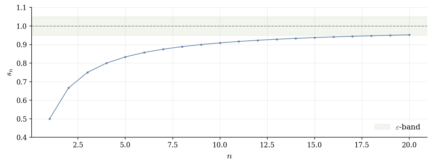
After n terms, we’ve filled s_n = \frac{1}{2} + \frac{1}{4} + \cdots + \frac{1}{2^n}.
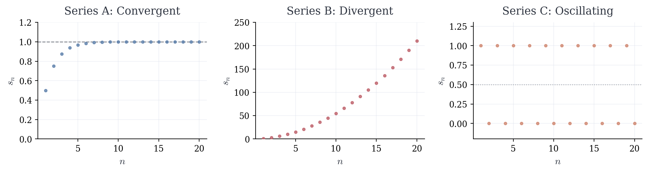
Compute the first few values: \begin{align*} s_1 &= \frac{1}{2} = 0.5 \\ s_2 &= \frac{1}{2} + \frac{1}{4} = \frac{3}{4}\\ s_3 &= \frac{3}{4} + \frac{1}{8} = \frac{7}{8} \\ s_4 &= \frac{7}{8} + \frac{1}{16} = \frac{15}{16} \end{align*}
Clearly s_n = 1 - \frac{1}{2^n}. As we add more terms, the unfilled portion shrinks—it’s always \frac{1}{2^n} of the square. Since \frac{1}{2^n} \to 0, the filled area approaches 1.
The geometry suggests a definite value: 1. But observe what we’ve actually done—we haven’t “summed infinitely many terms.” Instead, we’ve examined a sequence of finite sums: s_1, s_2, s_3, s_4, \ldots
This sequence converges to 1. The infinite sum, if it has meaning, should equal the limit of this sequence.
2.2.2 Series B
Now consider adding the positive integers: 1 + 2 + 3 + 4 + \cdots
Compute the finite sums: \begin{align*} s_1 &= 1 \\ s_2 &= 1 + 2 = 3 \\ s_3 &= 1 + 2 + 3 = 6 \\ s_4 &= 1 + 2 + 3 + 4 = 10 \\ s_5 &= 15, \quad s_6 = 21, \quad s_7 = 28, \ldots \end{align*}
The sequence of partial sums grows without bound. In fact, s_n = \frac{n(n+1)}{2}, which escapes to infinity. Unlike Series A, where contributions decay, here each new term is larger than the previous one. There is no mechanism for stabilization.
We cannot assign a finite value to this sum. The partial sums diverge.
2.2.3 Series C
Finally, consider the alternating sum: 1 - 1 + 1 - 1 + 1 - 1 + \cdots
The finite sums oscillate: \begin{align*} s_1 &= 1 \\ s_2 &= 1 - 1 = 0 \\ s_3 &= 1 - 1 + 1 = 1 \\ s_4 &= 1 - 1 + 1 - 1 = 0 \\ s_5 &= 1, \quad s_6 = 0, \quad s_7 = 1, \ldots \end{align*}
The sequence \{s_n\} bounces between two values indefinitely. Unlike Series B, which escapes to infinity, this sequence remains bounded. But it doesn’t approach any single value—for any proposed limit L and any tolerance \varepsilon, we can find arbitrarily large n where |s_n - L| \geq \varepsilon.
This is Euler’s problematic sum. The partial sums neither grow without bound nor converge to a limit. The classical framework cannot assign a value.
2.3 Finite Approximations
The three examples reveal a principle:
Series A has a natural value because its finite sums approach a limit
Series B has no finite value because its finite sums escape to infinity
Series C has no classical value because its finite sums oscillate
In each case, we examine the sequence of partial sums: s_1 = a_1, \quad s_2 = a_1 + a_2, \quad s_3 = a_1 + a_2 + a_3, \quad \ldots
The behavior of \{s_n\} determines whether the infinite sum has meaning. This observation—that infinite sums should be understood through finite approximations—is the foundational insight.
We already possess a complete theory of sequence convergence. We know precisely what it means for s_n \to L: for every \varepsilon > 0, there exists N such that |s_n - L| < \varepsilon for all n \geq N. The machinery is in place.
The strategy is to reduce infinite sums to sequence limits. An infinite sum “equals” L if the sequence of its partial sums converges to L. This transforms a new problem—what is infinite summation?—into a solved problem: sequence convergence.
2.4 Formal Definitions
Having motivated the approach through examples, we make it precise.
Definition 2.1 (Partial Sum) Let \{a_n\}_{n=1}^{\infty} be a sequence of real numbers. The nth partial sum is s_n = \sum_{k=1}^{n} a_k = a_1 + a_2 + \cdots + a_n.
The sequence \{s_n\}_{n=1}^{\infty} is called the sequence of partial sums.
The partial sum s_n represents what we’ve accumulated after n terms. It’s a finite sum—no infinite processes involved. The sequence \{s_n\} tracks how these finite approximations evolve.
Definition 2.2 (Series and Convergence) Let \{a_n\}_{n=1}^{\infty} be a sequence. We write \sum_{n=1}^{\infty} a_n to denote the infinite series with terms a_n.
The series converges to a sum S \in \mathbb{R} if the sequence of partial sums \{s_n\} converges to S. That is, if for every \varepsilon > 0, there exists N \in \mathbb{N} such that |s_n - S| < \varepsilon \quad \text{for all } n \geq N.
When this holds, we write \sum_{n=1}^{\infty} a_n = S and say the series converges to S, or that S is the sum of the series.
If the sequence \{s_n\} does not converge, the series diverges.
This definition accomplishes two things. First, it gives rigorous meaning to expressions involving infinitely many terms—not by performing infinite operations, but by examining limits of finite operations. Second, it reduces the study of series to the study of sequences, for which we already possess a complete theory.
Important: The notation \sum_{n=1}^{\infty} a_n plays a dual role. As a formal expression, it denotes the series itself—the process of forming partial sums. When the series converges, the same notation denotes the numerical value S. Context determines which meaning is intended.
Remark on Indexing: The starting index is arbitrary. We could equally well define \sum_{n=0}^{\infty} a_n (starting at n=0) or \sum_{n=k}^{\infty} a_n for any integer k. The theory remains identical. In specific examples, we choose the index that makes formulas cleanest.
2.5 When Partial Sums Have Closed Forms
The definition of convergence tells us what it means for a series to converge, but not how to determine convergence for specific series. In most cases, no explicit formula for s_n exists, and we must develop indirect tests.
However, certain special series admit closed-form expressions for their partial sums. For these, convergence analysis reduces to a sequence limit calculation. We examine the two most important classes: geometric and telescoping series.
2.6 Geometric Series
The geometric series is the most fundamental infinite sum in mathematics. It appears in compound interest, probability distributions, signal processing, quantum mechanics, and throughout analysis. Its complete characterization is explicit.
Definition 2.3 (Geometric Series) A geometric series has the form \sum_{n=0}^{\infty} ar^n = a + ar + ar^2 + ar^3 + \cdots where a, r \in \mathbb{R} with a \neq 0. The constant a is the first term and r is the common ratio.
Each term is obtained by multiplying the previous term by r. This multiplicative structure—constant ratio between consecutive terms—permits explicit analysis.
The approach is to find a formula for the nth partial sum: s_n = \sum_{k=0}^{n} ar^k = a + ar + ar^2 + \cdots + ar^n.
The technique involves multiplying by r to shift the entire sum by one position, then subtracting to eliminate all middle terms through systematic cancellation.
Lemma 2.1 (Geometric Partial Sum Formula) For r \neq 1, the nth partial sum of \sum_{k=0}^{\infty} ar^k is s_n = \sum_{k=0}^{n} ar^k = a\frac{1-r^{n+1}}{1-r}.
Proof.
Let s_n = a + ar + ar^2 + \cdots + ar^n. Multiply both sides by r: r s_n = ar + ar^2 + ar^3 + \cdots + ar^{n+1}.
Observe that r s_n contains almost all the same terms as s_n, shifted one position. Subtract: \begin{align*} s_n - r s_n &= (a + ar + ar^2 + \cdots + ar^n) - (ar + ar^2 + ar^3 + \cdots + ar^{n+1}) \\ &= a - ar^{n+1}. \end{align*}
Factor the left side: s_n(1-r) = a(1-r^{n+1}).
Provided r \neq 1, divide by (1-r): s_n = a\frac{1-r^{n+1}}{1-r}. \quad \square
This algebraic manipulation—multiply, shift, subtract—exploits the series’ self-similarity: multiplying by r reproduces almost the same series, differing only at the boundaries. This overlap creates systematic cancellation.
With the partial sum formula in hand, we determine convergence by examining \lim_{n \to \infty} s_n. The behavior depends entirely on r^{n+1}.
Theorem 2.1 (Convergence of Geometric Series) The geometric series \sum_{n=0}^{\infty} ar^n converges if and only if |r| < 1. When it converges, \sum_{n=0}^{\infty} ar^n = \frac{a}{1-r}.
If |r| \geq 1 and a \neq 0, the series diverges.
Proof.
We analyze the behavior of s_n = a\frac{1-r^{n+1}}{1-r} as n \to \infty by cases.
Case 1: |r| < 1.
From sequence theory, r^n \to 0 when |r| < 1 (exponential decay). Therefore r^{n+1} \to 0. Taking the limit: \lim_{n \to \infty} s_n = \lim_{n \to \infty} a\frac{1-r^{n+1}}{1-r} = a\frac{1-0}{1-r} = \frac{a}{1-r}.
To verify rigorously: given \varepsilon > 0, compute \left|s_n - \frac{a}{1-r}\right| = \left|a\frac{1-r^{n+1}}{1-r} - \frac{a}{1-r}\right| = \frac{|a|}{|1-r|} |r|^{n+1}.
Since |r| < 1, we have |r|^{n+1} \to 0. Choose N such that |r|^{n+1} < \frac{\varepsilon |1-r|}{|a|} for all n \geq N. Then for n \geq N, \left|s_n - \frac{a}{1-r}\right| = \frac{|a|}{|1-r|} |r|^{n+1} < \varepsilon.
Thus s_n \to \frac{a}{1-r}.
Case 2: |r| > 1 and a \neq 0.
Now |r|^{n+1} \to \infty. The terms |ar^n| = |a||r|^n grow without bound, so the series cannot converge.
Case 3: r = 1 and a \neq 0.
We have s_n = a(n+1) \to \pm\infty. The series diverges.
Case 4: r = -1 and a \neq 0.
The partial sums satisfy s_n = \begin{cases} a & n \text{ even} \\ 0 & n \text{ odd} \end{cases}
For any proposed limit L and \varepsilon = |a|/2, we can always find n large enough that |s_n - L| \geq \varepsilon. The sequence \{s_n\} does not converge.
Case 5: a = 0.
All terms vanish, so s_n = 0 for all n. The series converges to 0 trivially. \square
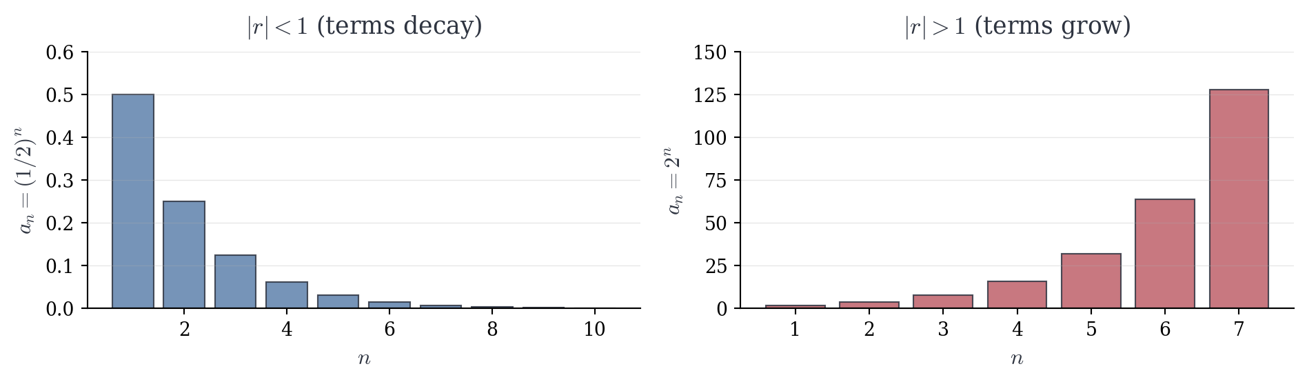
The theorem completely characterizes geometric series: convergence depends solely on whether |r| < 1. The ratio r controls whether terms decay fast enough for stabilization.
Geometric Interpretation: When |r| < 1, each term is a fraction of the previous—we add progressively smaller contributions. When |r| \geq 1, terms don’t shrink (or grow), and the sum escapes or oscillates.
Example 2.1 (Zeno’s Paradox) The series \sum_{n=1}^{\infty} \frac{1}{2^n} = \frac{1}{2} + \frac{1}{4} + \frac{1}{8} + \cdots is geometric with first term a = 1/2 and ratio r = 1/2. Since |r| = 1/2 < 1, \sum_{n=1}^{\infty} \frac{1}{2^n} = \frac{1/2}{1-1/2} = \frac{1/2}{1/2} = 1.
This resolves Zeno’s paradox. To walk one meter requires traveling \frac{1}{2} + \frac{1}{4} + \frac{1}{8} + \cdots = 1 \text{ meter} —exactly one meter, not “infinitely many pieces that never reach the goal.”
Zeno’s error: assuming infinitely many steps require infinite time. But if each step takes proportionally less time—if temporal intervals form the same geometric series—then total time is finite: \frac{t}{2} + \frac{t}{4} + \frac{t}{8} + \cdots = t.
Both spatial and temporal series converge together, i.e., motion is possible.
This resolution is not just philosophical. Continuous processes are constantly modeled by discrete approximations, and we must know when approximations converge to the thing approximated. Without geometric series, we couldn’t rigorously connect discrete measurements to continuous reality.
Example 2.2 (Repeating Decimals) Repeating decimals arise from geometric series. Consider 0.333\ldots: 0.333\ldots = 0.3 + 0.03 + 0.003 + \cdots = \sum_{n=1}^{\infty} \frac{3}{10^n}.
This is geometric with first term a = 3/10 and ratio r = 1/10. Since |r| < 1, \sum_{n=1}^{\infty} \frac{3}{10^n} = \frac{3/10}{1 - 1/10} = \frac{3/10}{9/10} = \frac{1}{3}.
Thus 0.333\ldots = 1/3.
Repeating decimals are not approximations—they are rational numbers in different form. The geometric series provides the conversion. Every repeating decimal corresponds to a convergent geometric series and thus to a rational number. Conversely, every rational number (in decimal form) either terminates or repeats, precisely because long division eventually cycles.
Example 2.3 (Divergence) The series \sum_{n=0}^{\infty} 2^n = 1 + 2 + 4 + 8 + \cdots has ratio r = 2 > 1, so it diverges. Partial sums grow exponentially s_n = \frac{1 - 2^{n+1}}{1-2} = 2^{n+1} - 1 \to \infty.
The series \sum_{n=0}^{\infty} (-1)^n = 1 - 1 + 1 - 1 + \cdots has ratio r = -1, so it diverges. This confirms our earlier observation—partial sums oscillate indefinitely.
2.7 Telescoping Series
Another class of series admits explicit partial sum formulas through systematic cancellation.
Definition 2.4 (Telescoping Series) A series of the form \sum_{n=1}^{\infty} (b_n - b_{n+1}) is called telescoping. Its partial sums satisfy s_n = \sum_{k=1}^{n} (b_k - b_{k+1}) = b_1 - b_{n+1}.
The name derives from the collapsing that occurs when we expand the sum: \begin{align*} s_n &= (b_1 - b_2) + (b_2 - b_3) + (b_3 - b_4) + \cdots + (b_n - b_{n+1}) \\ &= b_1 - \cancel{b_2} + \cancel{b_2} - \cancel{b_3} + \cancel{b_3} - \cancel{b_4} + \cdots + \cancel{b_n} - b_{n+1} \\ &= b_1 - b_{n+1}. \end{align*}
This explicit formula reduces convergence to a sequence limit.
Theorem 2.2 (Convergence of Telescoping Series) The series \sum_{n=1}^{\infty} (b_n - b_{n+1}) converges if and only if \lim_{n \to \infty} b_n exists. When it converges, \sum_{n=1}^{\infty} (b_n - b_{n+1}) = b_1 - \lim_{n \to \infty} b_n.
Proof.
From the telescoping property, s_n = b_1 - b_{n+1}.
Suppose b_n \to L. Let \varepsilon > 0. By convergence of \{b_n\}, there exists N such that |b_n - L| < \varepsilon for all n \geq N. Then for n \geq N, |s_n - (b_1 - L)| = |b_1 - b_{n+1} - b_1 + L| = |L - b_{n+1}| < \varepsilon.
Thus s_n \to b_1 - L.
Conversely, suppose s_n \to s. Since b_{n+1} = b_1 - s_n and s_n \to s, the limit laws give b_{n+1} \to b_1 - s. \square
The theorem shows that telescoping series converge precisely when the underlying sequence converges. The series value is determined by initial and limiting values.
:::{#exm-telescoping-partial-fractions} ### Partial Fractions
Consider \sum_{n=1}^{\infty} \frac{1}{n(n+1)}. To recognize this as telescoping, decompose via partial fractions.
Seek constants A, B such that \frac{1}{n(n+1)} = \frac{A}{n} + \frac{B}{n+1}.
Multiply by n(n+1): 1 = A(n+1) + Bn.
Setting n=0 gives A=1. Setting n=-1 gives B=-1. Therefore \frac{1}{n(n+1)} = \frac{1}{n} - \frac{1}{n+1}.
Verification.
\frac{1}{n} - \frac{1}{n+1} = \frac{(n+1) - n}{n(n+1)} = \frac{1}{n(n+1)}. \quad \square
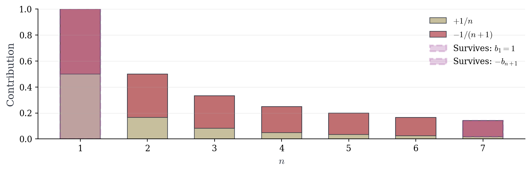
The series becomes \sum_{n=1}^{\infty} \left(\frac{1}{n} - \frac{1}{n+1}\right), which is telescoping with b_n = \frac{1}{n}. The partial sum is s_n = \frac{1}{1} - \frac{1}{n+1} = 1 - \frac{1}{n+1}.
Since \frac{1}{n+1} \to 0, we have s_n \to 1. The series converges to 1.
2.7.1 Logarithmic Telescoping
Consider \sum_{n=2}^{\infty} \ln\left(\frac{n-1}{n}\right). Using logarithm properties, \ln\left(\frac{n-1}{n}\right) = \ln(n-1) - \ln(n).
This is telescoping with b_n = \ln(n). Starting from n=2, the partial sum is \begin{align*} s_n &= [\ln(1) - \ln(2)] + [\ln(2) - \ln(3)] + \cdots + [\ln(n-1) - \ln(n)] \\ &= \ln(1) - \ln(n) \\ &= -\ln(n). \end{align*}
Since \ln(n) \to \infty, we have s_n \to -\infty. The series diverges.
2.8 A Necessary Condition for Convergence
We have seen series converge and diverge. A natural question: what can we say about the terms a_n when \sum a_n converges?
The partial sums s_n and s_{n-1} differ by a single term: a_n = s_n - s_{n-1}.
If \sum a_n converges, then s_n \to s for some s. Therefore s_{n-1} \to s as well (the sequence \{s_{n-1}\} is \{s_n\} shifted). By limit laws, a_n = s_n - s_{n-1} \to s - s = 0.
This observation is fundamental.
Theorem 2.3 (Necessary Condition for Convergence (Divergence Test)) If \sum_{n=1}^{\infty} a_n converges, then \lim_{n \to \infty} a_n = 0.
Equivalently, if a_n \not\to 0 or if \lim_{n \to \infty} a_n does not exist, then \sum_{n=1}^{\infty} a_n diverges.
Proof.
Suppose \sum_{n=1}^{\infty} a_n = s. Let s_n = \sum_{k=1}^{n} a_k. Then s_n \to s. For n \geq 1, a_n = s_n - s_{n-1}.
By limit laws, \lim_{n \to \infty} a_n = \lim_{n \to \infty} (s_n - s_{n-1}) = s - s = 0. \quad \square
The contrapositive provides a useful divergence test: if terms don’t approach zero, the series cannot converge.
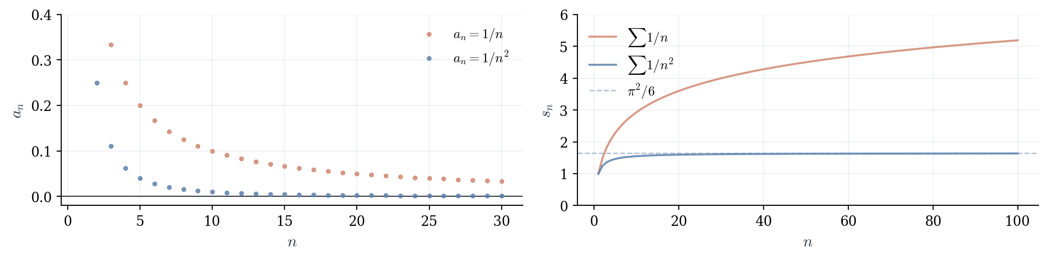
Warning. The converse is false. If a_n \to 0, the series may still diverge. The classic counterexample is the harmonic series \sum_{n=1}^{\infty} \frac{1}{n}, where \frac{1}{n} \to 0 but the series diverges (Theorem 3.5).
This theorem formalizes an intuitive principle: to accumulate to a finite total, contributions must eventually become negligible. If you keep adding 0.5 forever, the sum escapes. If terms merely shrink to 0.1, then 0.01, then 0.001, you’re still accumulating—just slowly. Convergence requires not just that terms shrink, but that accumulation decays.
The divergence test is a one-sided filter. It catches obviously divergent series (terms don’t vanish) but says nothing when terms do vanish. This asymmetry recurs: tests for divergence are often simpler than tests for convergence.
2.8.1 Examples
1. The series \sum_{n=1}^{\infty} \frac{n}{n+1} has terms a_n = \frac{n}{n+1} = \frac{1}{1 + 1/n} \to 1 \neq 0.
By the divergence test, the series diverges.
2. The series \sum_{n=1}^{\infty} \cos(n) has terms that oscillate and don’t converge to zero. The series diverges.
3. For \sum_{n=1}^{\infty} \frac{1}{n^2}, we have \frac{1}{n^2} \to 0. The divergence test provides no information. We cannot conclude convergence or divergence from this test alone. (This series converges, as the integral test will show.)
4. Consider \sum_{n=1}^{\infty} \frac{n+1}{2n}. We have a_n = \frac{n+1}{2n} = \frac{1 + 1/n}{2} \to \frac{1}{2} \neq 0.
The series diverges by the divergence test.