16 Parametric Curves and Vector-Valued Functions
16.1 Maps from \mathbb{R} to \mathbb{R}^k
In Calculus I, we studied functions f: \mathbb{R} \to \mathbb{R} and their derivatives as linear functionals. The differential df_a: \mathbb{R} \to \mathbb{R} was the unique linear map approximating f near a.
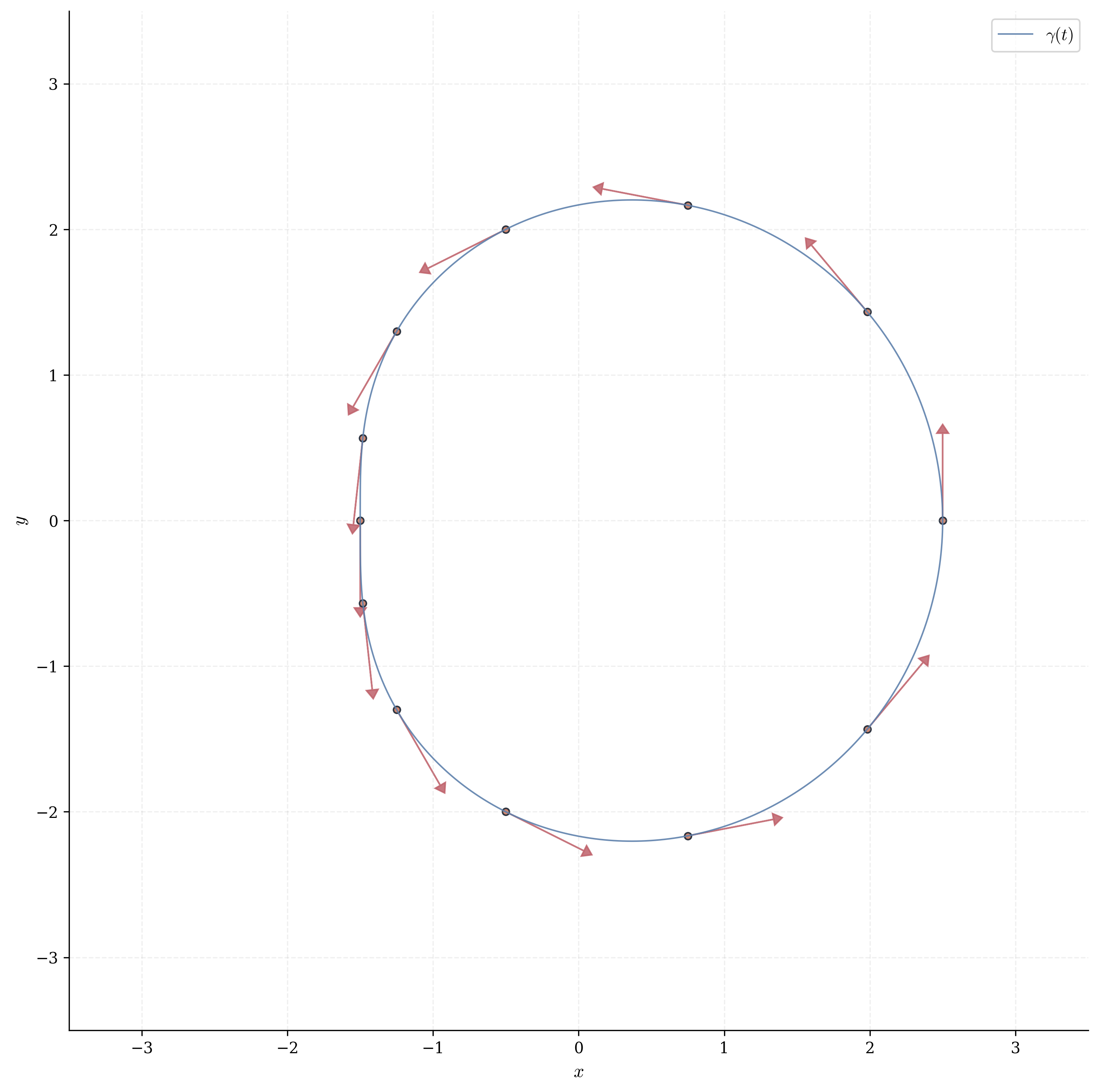
We now extend this framework to curves in space: maps \gamma: \mathbb{R} \to \mathbb{R}^k. Such maps assign to each parameter value t a point \gamma(t) \in \mathbb{R}^k. As t varies over an interval I, the image \gamma(I) traces a curve—though the same geometric curve can arise from infinitely many parametrizations.
A particle moving through space has position depending on time, \gamma(t) = (x(t), y(t), z(t)). The constraint y = f(x) is unnatural here—why privilege one coordinate over another? More fundamentally, many curves cannot be expressed as graphs: the circle x^2 + y^2 = 1 fails the vertical line test, yet we parametrize it as \gamma(t) = (\cos t, \sin t).
The derivative \gamma'(t) \in \mathbb{R}^k is the “velocity vector,” it lives in the tangent space at \gamma(t), pointing in the direction of motion with magnitude equal to speed. The differential d\gamma_t: \mathbb{R} \to \mathbb{R}^k is a linear map—the best linear approximation to \gamma near t. This recovers our earlier framework: when k = 1, we have d\gamma_t(h) = \gamma'(t) h, exactly the structure we studied for real-valued functions.
Definition 16.1 (Parametric Curve) A parametric curve in \mathbb{R}^k is a map \gamma: I \to \mathbb{R}^k where I \subseteq \mathbb{R} is an interval. We write: \gamma(t) = (x_1(t), \ldots, x_k(t)) where each component x_i: I \to \mathbb{R} is C^1 (continuously differentiable). The image \gamma(I) \subseteq \mathbb{R}^k is the geometric curve traced by the parametrization.
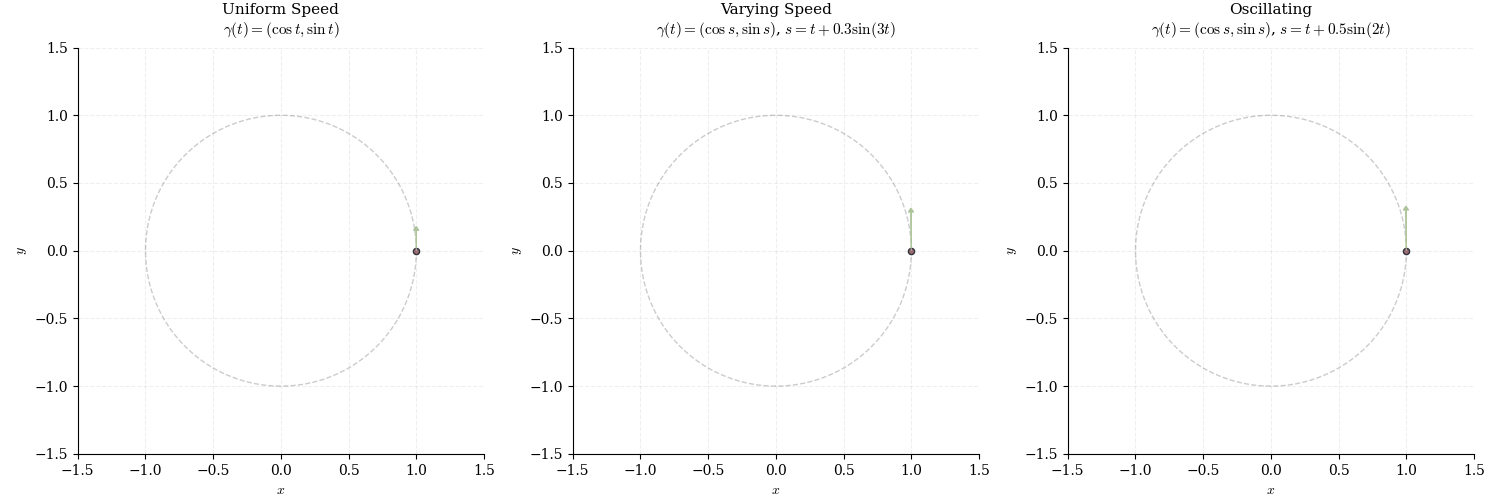
Distinct parametrizations may trace the same geometric curve. The circle admits \gamma(t) = (\cos t, \sin t) and \tilde{\gamma}(t) = (\cos(2t), \sin(2t))—the latter traverses twice as fast. This distinction between parametrized curve (the map \gamma) and geometric curve (the image \gamma(I)) is essential: physics depends on parametrization (velocity requires a time coordinate), while geometry does not (curvature is intrinsic to the shape).
Example 16.1 (Circle) The unit circle x^2 + y^2 = 1 has parametrization: \gamma(t) = (\cos t, \sin t), \quad t \in [0, 2\pi). As t increases from 0 to 2\pi, the point \gamma(t) traces the circle counterclockwise from (1, 0).
Example 16.2 (Helix) The curve \gamma(t) = (a\cos t, a\sin t, bt), \quad t \in \mathbb{R} winds around a cylinder of radius a while ascending at rate b. Projecting onto the xy-plane yields a circle; projecting onto the z-axis yields a line. The helix interpolates between these extremes—a fundamentally three-dimensional object (DNA double helix, screw threads, Archimedean spirals).
Example 16.3 (Cycloid) A point on the rim of a wheel of radius a rolling along the x-axis traces: \gamma(t) = (a(t - \sin t), a(1 - \cos t)), \quad t \geq 0. This solves the brachistochrone problem: among all curves connecting two points, the cycloid minimizes descent time under gravity alone. The solution involves variational calculus—the Euler-Lagrange equation applied to the time functional.
16.2 Componentwise Differentiation
Recall that if L: \mathbb{R}^n \to \mathbb{R}^m is linear, then L is determined by its action on basis vectors. For curves \gamma: \mathbb{R} \to \mathbb{R}^k, the differential d\gamma_t: \mathbb{R} \to \mathbb{R}^k must be linear, hence determined by its value on 1 \in \mathbb{R}. This forces componentwise differentiation.
Definition 16.2 (Derivative of Parametric Curve) If \gamma: I \to \mathbb{R}^k is differentiable at t_0, its derivative is \gamma'(t_0) = \lim_{h \to 0} \frac{\gamma(t_0 + h) - \gamma(t_0)}{h} = (x_1'(t_0), \ldots, x_k'(t_0)) \in \mathbb{R}^k.
The differential d\gamma_t: \mathbb{R} \to \mathbb{R}^k is the linear map defined by: d\gamma_t(h) = \gamma'(t) \cdot h.
This is the multidimensional analogue of our earlier definition. For f: \mathbb{R} \to \mathbb{R}, we had df_a(h) = f'(a) h. Now \gamma'(t) is a vector in \mathbb{R}^k, and d\gamma_t(h) is scalar multiplication: h \mapsto h \gamma'(t).
The differential d\gamma_t approximates \gamma near t linearly \gamma(t + h) \approx \gamma(t) + d\gamma_t(h) = \gamma(t) + \gamma'(t) h. The vector \gamma'(t) \in \mathbb{R}^k is tangent to the curve at \gamma(t): it points in the direction of increasing t, with magnitude measuring the rate of change. When the parameter is time, \gamma'(t) is the velocity vector.
Represent d\gamma_t as a k \times 1 matrix (a column vector): d\gamma_t = \begin{pmatrix} x_1'(t) \\ \vdots \\ x_k'(t) \end{pmatrix}. For h \in \mathbb{R}, matrix multiplication gives d\gamma_t(h) = h \cdot \gamma'(t), exactly the definition. This is the Jacobian matrix of \gamma—though we defer general treatment to multivariable calculus.
Example 16.4 (Helix Velocity) For the helix \gamma(t) = (a\cos t, a\sin t, bt): \gamma'(t) = (-a\sin t, a\cos t, b). Decompose this velocity:
Horizontal component (-a\sin t, a\cos t, 0) lies tangent to the circle x^2 + y^2 = a^2 (perpendicular to radius \vec{OP} = (a\cos t, a\sin t, 0)).
Vertical component (0, 0, b) is constant, yielding uniform ascent.
The speed is: \|\gamma'(t)\| = \sqrt{a^2\sin^2 t + a^2\cos^2 t + b^2} = \sqrt{a^2 + b^2}. Despite changing direction continuously, the helix maintains constant speed—a uniform motion along a non-geodesic path. Only helices and circles have this property (among smooth curves).
16.3 Arc Length
In \mathbb{R}^k, distance is measured by the Euclidean norm: \|\mathbf{v}\| = \sqrt{v_1^2 + \cdots + v_k^2}. For a curve \gamma: [a,b] \to \mathbb{R}^k, we seek the total distance traversed as t ranges from a to b. This cannot depend on parametrization—reparametrizing by s = \phi(t) should preserve length.
Partition [a,b] into n subintervals [t_{i-1}, t_i] with \Delta t_i = t_i - t_{i-1}. Approximate the curve by the polygonal path connecting consecutive points \gamma(t_i). The length of the i-th segment is: \|\gamma(t_i) - \gamma(t_{i-1})\| = \left\|\frac{\gamma(t_i) - \gamma(t_{i-1})}{\Delta t_i}\right\| \Delta t_i \approx \|\gamma'(t_i^*)\| \Delta t_i by the definition of derivative. Summing over all segments: L \approx \sum_{i=1}^n \|\gamma'(t_i^*)\| \Delta t_i. As \max \Delta t_i \to 0, this Riemann sum converges to an integral.
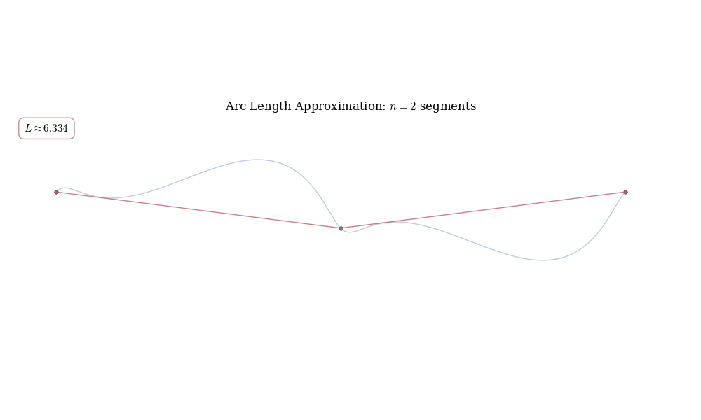
Definition 16.3 (Arc Length) For a C^1 curve \gamma: [a,b] \to \mathbb{R}^k, the arc length is L(\gamma) = \int_a^b \|\gamma'(t)\| \, dt. In coordinates, if \gamma(t) = (x_1(t), \ldots, x_k(t)): L(\gamma) = \int_a^b \sqrt{\sum_{i=1}^k (x_i'(t))^2} \, dt.
Unification with Graphs. For curves y = f(x) on [a,b], parametrize by \gamma(x) = (x, f(x)). Then \gamma'(x) = (1, f'(x)), so: \|\gamma'(x)\| = \sqrt{1 + (f'(x))^2}, recovering the formula from Calculus I. The parametric viewpoint reveals this as a special case: graphs are curves constrained to move rightward at unit speed in the x-direction.
Example 16.5 (Arc Length of Helix) For the helix \gamma(t) = (a\cos t, a\sin t, bt) on t \in [0, 2\pi]: \|\gamma'(t)\| = \sqrt{a^2 + b^2} \quad \text{(constant speed)}, so: L = \int_0^{2\pi} \sqrt{a^2 + b^2} \, dt = 2\pi\sqrt{a^2 + b^2}. The factor \sqrt{a^2 + b^2} is the hypotenuse of a right triangle with legs a (horizontal speed) and b (vertical speed). Unwrap the cylinder: the helix becomes a straight line of slope b/a, and the length formula reduces to Pythagoras.
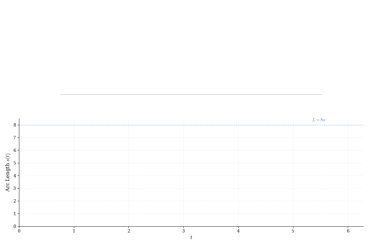
Example 16.6 (Arc Length of Cycloid) For one arch of the cycloid \gamma(t) = (a(t - \sin t), a(1 - \cos t)) on t \in [0, 2\pi]: \gamma'(t) = (a(1 - \cos t), a\sin t). Compute the speed using the identity 1 - \cos t = 2\sin^2(t/2): \|\gamma'(t)\|^2 = a^2(1 - \cos t)^2 + a^2\sin^2 t = a^2(2 - 2\cos t) = 4a^2\sin^2\frac{t}{2}, so \|\gamma'(t)\| = 2a|\sin(t/2)|. For t \in [0, 2\pi], the sine is nonnegative: L = \int_0^{2\pi} 2a\sin\frac{t}{2} \, dt = 2a \cdot \left[-2\cos\frac{t}{2}\right]_0^{2\pi} = 4a[1 - (-1)] = 8a. Remarkably, the arc length is exactly 8a—independent of \pi. This transcendental curve has an algebraic length, a surprise known to Galileo and formalized by Roberval (1634).
16.4 The Cross Product in \mathbb{R}^3
16.4.1 Definition and Properties
The cross product \mathbf{a} \times \mathbf{b} is a bilinear operation defined only in \mathbb{R}^3. Given vectors \mathbf{a} = \begin{pmatrix} a_1 \\ a_2 \\ a_3 \end{pmatrix} and \mathbf{b} = \begin{pmatrix} b_1 \\ b_2 \\ b_3 \end{pmatrix}, their cross product is the vector: \mathbf{a} \times \mathbf{b} = \begin{pmatrix} a_2b_3 - a_3b_2 \\ a_3b_1 - a_1b_3 \\ a_1b_2 - a_2b_1 \end{pmatrix}.
This can be computed using the determinant formula: \mathbf{a} \times \mathbf{b} = \begin{vmatrix} \mathbf{e}_1 & \mathbf{e}_2 & \mathbf{e}_3 \\ a_1 & a_2 & a_3 \\ b_1 & b_2 & b_3 \end{vmatrix} where \mathbf{e}_1, \mathbf{e}_2, \mathbf{e}_3 are the standard basis vectors and we expand along the first row.
Key Properties:
Antisymmetry: \mathbf{a} \times \mathbf{b} = -(\mathbf{b} \times \mathbf{a}).
Orthogonality: \mathbf{a} \times \mathbf{b} is perpendicular to both \mathbf{a} and \mathbf{b}. Verify: (\mathbf{a} \times \mathbf{b}) \cdot \mathbf{a} = 0 and (\mathbf{a} \times \mathbf{b}) \cdot \mathbf{b} = 0.
Magnitude: \|\mathbf{a} \times \mathbf{b}\| = \|\mathbf{a}\| \|\mathbf{b}\| \sin\theta, where \theta is the angle between \mathbf{a} and \mathbf{b}. This equals the area of the parallelogram spanned by \mathbf{a} and \mathbf{b}.
Bilinearity: The cross product is linear in each argument: (\alpha\mathbf{a} + \beta\mathbf{a}') \times \mathbf{b} = \alpha(\mathbf{a} \times \mathbf{b}) + \beta(\mathbf{a}' \times \mathbf{b}).
Why only \mathbb{R}^3? The cross product is intimately tied to the dimension. There exists a “cross product-like” operation only in dimensions 3 and 7 (related to octonions). In \mathbb{R}^2, we can define the scalar cross product (a_1, a_2) \times (b_1, b_2) = a_1b_2 - a_2b_1 (the signed area). In higher dimensions, the cross product fails to exist—though the wedge product generalizes the core ideas.
Example 16.7 (Cross Product) Compute \mathbf{a} \times \mathbf{b} for \mathbf{a} = \begin{pmatrix} 1 \\ 2 \\ 3 \end{pmatrix} and \mathbf{b} = \begin{pmatrix} 4 \\ 5 \\ 6 \end{pmatrix}: \mathbf{a} \times \mathbf{b} = \begin{vmatrix} \mathbf{e}_1 & \mathbf{e}_2 & \mathbf{e}_3 \\ 1 & 2 & 3 \\ 4 & 5 & 6 \end{vmatrix} = \mathbf{e}_1(2 \cdot 6 - 3 \cdot 5) - \mathbf{e}_2(1 \cdot 6 - 3 \cdot 4) + \mathbf{e}_3(1 \cdot 5 - 2 \cdot 4) = \mathbf{e}_1(-3) - \mathbf{e}_2(-6) + \mathbf{e}_3(-3) = \begin{pmatrix} -3 \\ 6 \\ -3 \end{pmatrix}. Verify orthogonality: \mathbf{a} \cdot (\mathbf{a} \times \mathbf{b}) = 1(-3) + 2(6) + 3(-3) = -3 + 12 - 9 = 0. Similarly, \mathbf{b} \cdot (\mathbf{a} \times \mathbf{b}) = 0.
16.4.2 Geometric Applications
The cross product encodes geometry in \mathbb{R}^3:
Torque: In physics, torque \boldsymbol{\tau} = \mathbf{r} \times \mathbf{F} measures the rotational effect of force \mathbf{F} applied at position \mathbf{r} relative to a pivot. The magnitude \|\boldsymbol{\tau}\| = \|\mathbf{r}\| \|\mathbf{F}\| \sin\theta captures the lever-arm principle.
Angular Momentum: For a particle with momentum \mathbf{p} at position \mathbf{r}, angular momentum is \mathbf{L} = \mathbf{r} \times \mathbf{p}. Conservation of \mathbf{L} (when torque vanishes) governs planetary motion and spinning tops.
Normal Vectors: The cross product of two tangent vectors to a surface yields a normal vector. For the plane spanned by \mathbf{a} and \mathbf{b}, the normal is \mathbf{n} = \mathbf{a} \times \mathbf{b}.
The cross product is a special case of the wedge product \mathbf{a} \wedge \mathbf{b}, which exists in all dimensions and underlies exterior algebra (Grassmann algebra). While we cannot develop this theory here, the essential idea is:
In \mathbb{R}^n, the wedge product \mathbf{a} \wedge \mathbf{b} is a 2-vector (or bivector)—an object representing the oriented plane spanned by \mathbf{a} and \mathbf{b}. It satisfies:
Antisymmetry: \mathbf{a} \wedge \mathbf{b} = -(\mathbf{b} \wedge \mathbf{a}).
Area: \|\mathbf{a} \wedge \mathbf{b}\| equals the area of the parallelogram.
Associativity: (\mathbf{a} \wedge \mathbf{b}) \wedge \mathbf{c} = \mathbf{a} \wedge (\mathbf{b} \wedge \mathbf{c}) (the cross product is not associative).
Why does \mathbb{R}^3 get vectors? The space of 2-vectors in \mathbb{R}^3 is 3-dimensional (spanned by e_1 \wedge e_2, e_2 \wedge e_3, e_3 \wedge e_1), matching the dimension of \mathbb{R}^3 itself. This allows us to identify 2-vectors with ordinary vectors via the Hodge star operator: \star(\mathbf{a} \wedge \mathbf{b}) = \mathbf{a} \times \mathbf{b}. This identification is unique to dimension 3. In other dimensions, 2-vectors remain genuinely distinct from vectors.
The cross product inherits the wedge product’s antisymmetry and geometric meaning (oriented area), but loses associativity. In higher dimensions, exterior algebra—formalized by Grassmann (1844) and refined by Cartan—is essential for differential geometry, differential forms, integration on manifolds, and Maxwell’s equations.
Further Study: For rigorous treatment, consult:
Walter Rudin, Principles of Mathematical Analysis: Discusses differential forms and the exterior derivative.
Michael Spivak, Calculus on Manifolds: Develops exterior algebra from scratch, culminating in Stokes’ theorem.
John M. Lee, Introduction to Smooth Manifolds: Modern differential geometry perspective.
The wedge product is to the cross product as linear algebra is to 3D geometry.
16.5 Curvature
16.5.1 From Graphs to Curves
In Calculus I, we defined curvature \kappa = |f''(x)|/(1 + (f'(x))^2)^{3/2} for graphs y = f(x). This measured how quickly the tangent line rotates per unit arc length. For parametric curves, we seek an intrinsic definition—independent of both parametrization and coordinate system.
The unit tangent vector \mathbf{T}(t) = \gamma'(t)/\|\gamma'(t)\| has constant norm 1 and points in the direction of motion. As we traverse the curve, \mathbf{T} rotates: the rate of this rotation, measured per unit arc length, is the curvature.
Definition 16.4 (Curvature) For a C^2 curve \gamma: I \to \mathbb{R}^k with \gamma'(t) \neq 0, the curvature at t is \kappa(t) = \frac{\|\gamma'(t) \times \gamma''(t)\|}{\|\gamma'(t)\|^3}.
In \mathbb{R}^2, interpret the cross product as the scalar: (x', y') \times (x'', y'') = x'y'' - y'x''.
Derivation. Let s(t) = \int_0^t \|\gamma'(\tau)\| \, d\tau be the arc length function. Then ds/dt = \|\gamma'\|, and by the chain rule: \mathbf{T} = \frac{\gamma'}{\|\gamma'\|} = \frac{d\gamma/dt}{ds/dt} = \frac{d\gamma}{ds}. Differentiating with respect to t: \frac{d\mathbf{T}}{dt} = \frac{d^2\gamma}{ds^2} \cdot \frac{ds}{dt} = \kappa \mathbf{N} \cdot \|\gamma'\| where \mathbf{N} is the unit normal and \kappa = \|d\mathbf{T}/ds\| (the rotation rate per unit arc length). Solving: \kappa = \frac{\|d\mathbf{T}/dt\|}{\|\gamma'\|}. A calculation using the product rule on \mathbf{T} = \gamma'/\|\gamma'\| yields the cross product formula.
The curvature \kappa measures bending intensity. A straight line has \kappa = 0 (no rotation); a circle of radius r has \kappa = 1/r (constant bending inversely proportional to size). At each point, the osculating circle—the unique circle matching both position, tangent, and curvature—has radius R = 1/\kappa.
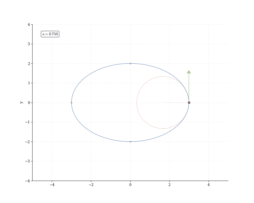
Example 16.8 (Curvature of Circle) For the circle \gamma(t) = (a\cos t, a\sin t): \gamma'(t) = (-a\sin t, a\cos t), \quad \gamma''(t) = (-a\cos t, -a\sin t). The 2D cross product is: \gamma' \times \gamma'' = (-a\sin t)(-a\sin t) - (a\cos t)(-a\cos t) = a^2. Thus: \kappa = \frac{|a^2|}{a^3} = \frac{1}{a}. Curvature is constant (as expected for a circle) and inversely proportional to radius: smaller circles bend more sharply.
16.6 Applications to Physics: Kepler’s Laws
16.6.1 Newton’s Gravitational Equation
In Calculus I, we analyzed Kepler’s ellipses using implicit differentiation. Now we derive the orbit equation directly from Newton’s law.
A planet of mass m at position \gamma(t) \in \mathbb{R}^3 experiences gravitational force from a star of mass M at the origin: \mathbf{F} = -\frac{GMm}{\|\gamma\|^3}\gamma. The force points toward the origin (attractive, hence negative sign) with magnitude GMm/\|\gamma\|^2 (inverse-square law). Newton’s second law \mathbf{F} = m\gamma'' gives: \gamma''(t) = -\frac{GM}{\|\gamma(t)\|^3}\gamma(t). This is a second-order nonlinear vector ODE. Its solutions are conic sections—ellipses (bound orbits), parabolas (escape trajectories), or hyperbolas (scattering trajectories)—depending on total energy.
Kepler’s Second Law states that the radius vector sweeps equal areas in equal times. Define the angular momentum: \mathbf{L}(t) = \gamma(t) \times \gamma'(t). Differentiating (using the product rule for cross products): \frac{d\mathbf{L}}{dt} = \gamma' \times \gamma' + \gamma \times \gamma'' = 0 + \gamma \times \left(-\frac{GM}{\|\gamma\|^3}\gamma\right) = 0 since \gamma \times \gamma = 0 (a vector is parallel to itself). Thus \mathbf{L} is constant—conservation of angular momentum.
The constancy of \mathbf{L} implies the orbit lies in a plane perpendicular to \mathbf{L}. In this plane, the area swept out in time dt is (1/2)\|\gamma \times \gamma'\| dt = (1/2)\|\mathbf{L}\| dt, proportional to dt alone. Equal times yield equal areas—Kepler’s Second Law emerges from the 1/r^2 force law via calculus.
16.7 Line Integrals
16.7.1 Scalar Fields
Beyond arc length, we integrate functions along curves. Given a scalar field f: \mathbb{R}^k \to \mathbb{R} and a path \gamma: [a,b] \to \mathbb{R}^k, partition the parameter interval and form the Riemann sum: \sum_{i=1}^n f(\gamma(t_i^*)) \|\gamma'(t_i^*)\| \Delta t_i. Each term approximates the contribution from a small arc segment: f evaluated at a point times the arc length \|\gamma'\| \Delta t of that segment. Taking the limit:
Definition 16.5 (Scalar Line Integral) For f: \mathbb{R}^k \to \mathbb{R} continuous and \gamma: [a,b] \to \mathbb{R}^k a C^1 path, the line integral is: \int_\gamma f \, ds = \int_a^b f(\gamma(t)) \|\gamma'(t)\| \, dt.
Physical Interpretation. If f(\mathbf{x}) represents mass density at point \mathbf{x}, then \int_\gamma f \, ds is the total mass of a wire shaped like \gamma. If f is temperature, the integral measures “thermal content” along the path. The element ds = \|\gamma'\| dt is the infinitesimal arc length.
16.8 Arc Length Parameterization
16.8.1 Unit Speed Curves
A curve is parameterized by arc length if \|\gamma'(s)\| = 1 for all s. In this natural parametrization, the parameter s measures distance: moving from s = s_0 to s = s_1 traverses exactly |s_1 - s_0| units of length.
Given \gamma(t) with arbitrary parametrization, reparametrize by arc length:
Define the arc length function: s(t) = \int_0^t \|\gamma'(\tau)\| \, d\tau.
Invert to obtain t = t(s) (assuming \gamma'(t) \neq 0).
Compose: \tilde{\gamma}(s) = \gamma(t(s)).
Then \|\tilde{\gamma}'(s)\| = 1 by construction (verify using the chain rule).
Why is this useful? In the arc length parameterization:
Curvature simplifies: \kappa = \|\tilde{\gamma}''(s)\| (no denominator).
The second derivative \tilde{\gamma}''(s) \perp \tilde{\gamma}'(s) always (since \|\tilde{\gamma}'\|^2 = 1 is constant, differentiating gives 2\tilde{\gamma}' \cdot \tilde{\gamma}'' = 0).
Arc length parametrization is intrinsic—it depends only on the geometric curve, not on our choice of parameter. This is the natural setting for differential geometry: studying shapes independently of how we describe them.
For a unit-speed curve \gamma(s) in \mathbb{R}^3 with \kappa(s) > 0, define the Frenet frame: - Unit tangent: \mathbf{T}(s) = \gamma'(s) (direction of motion).
Principal normal: \mathbf{N}(s) = \mathbf{T}'(s)/\|\mathbf{T}'(s)\| (direction curve bends toward).
Binormal: \mathbf{B}(s) = \mathbf{T}(s) \times \mathbf{N}(s) (perpendicular to osculating plane).
These three orthonormal vectors satisfy the Frenet-Serret formulas: \begin{aligned} \mathbf{T}' &= \kappa \mathbf{N}, \\ \mathbf{N}' &= -\kappa \mathbf{T} + \tau \mathbf{B}, \\ \mathbf{B}' &= -\tau \mathbf{N}, \end{aligned} where \kappa(s) = \|\mathbf{T}'(s)\| is curvature and \tau(s) = -\mathbf{B}'(s) \cdot \mathbf{N}(s) is torsion (rate of twisting out of the osculating plane).
Fundamental Theorem of Space Curves. Given continuous functions \kappa(s) > 0 and \tau(s), there exists a unique curve \gamma(s) (up to rigid motion) with these curvature and torsion functions. The functions (\kappa, \tau) completely determine the curve’s shape—analogous to how f'' determines f up to affine transformations in 1D.
For the helix \gamma(s) = (a\cos(s/c), a\sin(s/c), bs/c) where c = \sqrt{a^2 + b^2}, both \kappa and \tau are constant: \kappa = \frac{a}{a^2 + b^2}, \quad \tau = \frac{b}{a^2 + b^2}. This explains why springs have predictable mechanical properties: their geometry is determined by two constants alone.
This framework extends to surfaces via Gaussian curvature (Gauss’s Theorema Egregium) and higher-dimensional Riemannian manifolds.
Parametrize the ellipse x^2/a^2 + y^2/b^2 = 1 as \mathbf{r}(t) = (a\cos t, b\sin t), t \in [0, 2\pi]. Show that the arc length is: L = 4a\int_0^{\pi/2} \sqrt{1 - e^2\sin^2\theta} \, d\theta where e = \sqrt{1 - b^2/a^2} is the eccentricity. This integral (an elliptic integral) has no elementary antiderivative.
The parametric curve \mathbf{r}(t) = (A\sin(at + \delta), B\sin(bt)) produces intricate patterns depending on the ratio a/b. Plot several examples and compute their curvature. When is \kappa constant?
The curve \mathbf{r}(t) = (a\cos^3 t, a\sin^3 t), t \in [0, 2\pi], is the astroid—the path traced by a point on a small circle rolling inside a larger circle. Find its arc length and identify the points of maximum curvature.
Verify that \mathbf{r}(t) = (a\cos\theta(t), b\sin\theta(t)) satisfies \mathbf{r}'' = -k\mathbf{r}/r^3 if and only if \theta(t) satisfies a specific differential equation. (This is the equation of the orbit in classical mechanics.)
Show that for any force \mathbf{F}(\mathbf{r}) = f(r)\hat{\mathbf{r}} (where f depends only on distance r = \|\mathbf{r}\|), the work integral \int_C \mathbf{F} \cdot d\mathbf{r} is path-independent—it depends only on the initial and final positions, not on the curve connecting them. (Hint: show \mathbf{F} = -\nabla U for some potential U(r).)