8 The Riemann Integral

8.1 From Rates to Accumulation

Differentiation answers: given f, what is the instantaneous rate of change at a? The differential df_a(h) = f'(a)h gives the best linear approximation to how f changes.

Integration reverses this question: given rates of change everywhere, what is the total change? If you know velocity at each instant, how far did you travel? If marginal cost per unit is specified, what’s the total cost of production?

The geometric manifestation is immediate: how do we measure area under a curve?

8.2 The Area Problem

For rectangles, triangles, circles—shapes with symmetry—area reduces to algebra. But consider the region under y = f(x) from x = a to x = b.

When f is constant, we have a rectangle: area = f(a)(b-a). When f varies—even for f(x) = x^2—no elementary formula exists. The boundary curves, and geometry fails us.

The resolution parallels our approach to series (Section 2.1). Archimedes trapped areas between inscribed and circumscribed polygons, forcing convergence between bounds—exactly like upper and lower sums.

Newton and Leibniz discovered the Fundamental Theorem, connecting integration to antidifferentiation. But Riemann (1854) provided the foundation: define the integral as a limit of approximating sums, just as we defined series via partial sums (Section 2.4).

We develop Darboux’s streamlined approach first, then show equivalence to Riemann sums.

8.3 Partitions

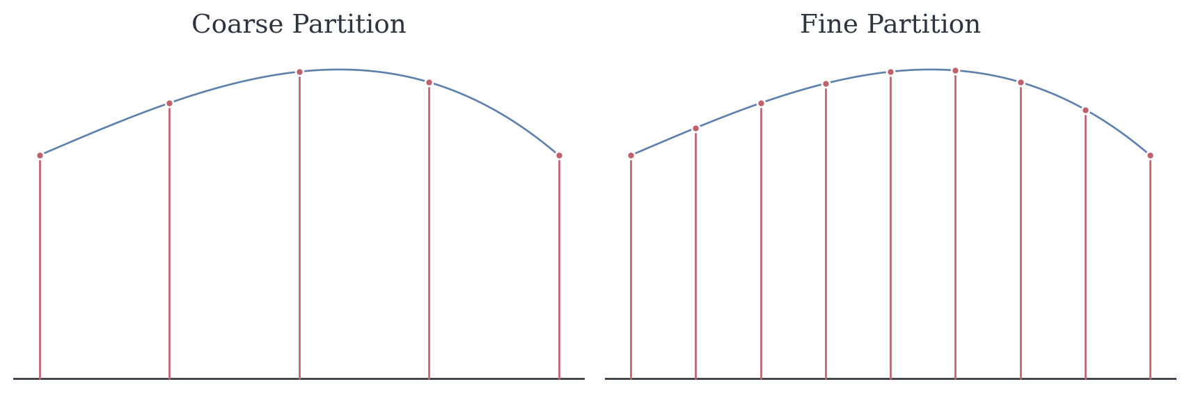
To approximate area under f on [a,b], subdivide the interval into pieces.

Definition 8.1 (Partition) A partition of [a,b] is a finite set P = \{x_0, x_1, \ldots, x_n\} with a = x_0 < x_1 < \cdots < x_n = b.

The mesh of P is \|P\| = \max_{i} (x_i - x_{i-1}), the longest subinterval length.

Smaller mesh means finer resolution. Adding points creates a refinement—it can only decrease the mesh.

8.4 Extremal Values

To approximate area over [x_{i-1}, x_i], we need the “best” and “worst” behavior of f there. But extrema might not be attained—consider f(x) = x on (0,1). As x \to 0^+, we have f(x) \to 0, but f never equals 0 on (0,1).

We need bounds that don’t require attainment.

Definition 8.2 (Supremum and Infimum) For nonempty S \subset \mathbb{R} bounded above, \sup S is the least upper bound: it’s an upper bound, and no smaller number works. Similarly, \inf S is the greatest lower bound when S is bounded below.

Maximum/minimum require attainment. Supremum/infimum are the tightest possible bounds, attained or not. By completeness of \mathbb{R} (Theorem 3.4), they always exist for bounded sets.

8.5 Upper and Lower Sums

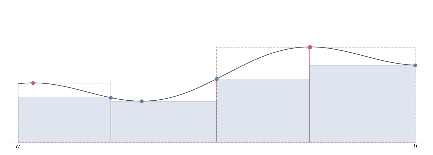
Let f : [a,b] \to \mathbb{R} be bounded. Given partition P, on each subinterval [x_{i-1}, x_i] define m_i = \inf\{f(x) : x \in [x_{i-1}, x_i]\}, \quad M_i = \sup\{f(x):x \in [x_{i-1}, x_i]\}.

Definition 8.3 (Upper and Lower Sums) L(f, P) = \sum_{i=1}^{n} m_i (x_i - x_{i-1}), \quad U(f, P) = \sum_{i=1}^{n} M_i (x_i - x_{i-1}).

Geometrically: L(f,P) uses inscribed rectangles (smallest possible heights), U(f,P) uses circumscribed rectangles (largest possible heights). Since m_i \leq M_i, we always have L(f, P) \leq U(f, P).

The true area must lie between these bounds.

8.6 Refinement

Adding points improves our bounds. Lower sums increase (we’re not stuck with worst underestimates over large intervals), upper sums decrease.

Refinement of partitions showing upper and lower sums converging

Proof.

It suffices to consider the case where Q contains exactly one more point than P. The general result follows by induction on the number of additional points.

Let P = \{x_0, x_1, \ldots, x_n\} and suppose Q adds a single point t with x_{j-1} < t < x_j for some j. Then Q = \{x_0, \ldots, x_{j-1}, t, x_j, \ldots, x_n\}.

For i \neq j, the i-th subinterval is unchanged, so the corresponding terms in L(f,P) and L(f,Q) coincide. The difference lies in how we handle [x_{j-1}, x_j].

In P, this interval contributes m_j(x_j - x_{j-1}) \quad \text{where } m_j = \inf\{f(x) : x \in [x_{j-1}, x_j]\}.

In Q, we split this into two pieces: [x_{j-1}, t] and [t, x_j], contributing m_j'(t - x_{j-1}) + m_j''(x_j - t) where m_j' = \inf\{f(x) : x \in [x_{j-1}, t]\}, \quad m_j'' = \inf\{f(x) : x \in [t, x_j]\}.

Since [x_{j-1}, t] \subseteq [x_{j-1}, x_j] and [t, x_j] \subseteq [x_{j-1}, x_j], we have m_j \leq m_j' \quad \text{and} \quad m_j \leq m_j''.

Therefore, \begin{align*} m_j'(t - x_{j-1}) + m_j''(x_j - t) &\geq m_j(t - x_{j-1}) + m_j(x_j - t) \\ &= m_j(x_j - x_{j-1}). \end{align*}

This shows L(f, P) \leq L(f, Q).

For upper sums, let M_j = \sup\{f(x) : x \in [x_{j-1}, x_j]\}, M_j' = \sup\{f(x) : x \in [x_{j-1}, t]\}, \quad M_j'' = \sup\{f(x) : x \in [t, x_j]\}.

Then M_j \geq M_j' and M_j \geq M_j'', giving \begin{align*} M_j'(t - x_{j-1}) + M_j''(x_j - t) &\leq M_j(t - x_{j-1}) + M_j(x_j - t) \\ &= M_j(x_j - x_{j-1}). \end{align*}

Thus U(f, Q) \leq U(f, P).

Finally, since m_i \leq M_i on every subinterval, we have L(f, Q) \leq U(f, Q). \square

The refinement theorem tells us that as we add more points, lower sums never decrease and upper sums never increase. But there’s a structural property: any lower sum is bounded above by any upper sum, even when they come from completely different partitions. This is not obvious—it doesn’t follow immediately from the definition. Yet it’s this property that makes the entire theory work. To see why, consider that we’re trying to define a single number (the integral) as both the supremum of all lower sums and the infimum of all upper sums. For these to potentially agree, the set of lower sums must lie entirely below the set of upper sums. Otherwise, we might have a lower sum larger than an upper sum, making it impossible for their supremum and infimum to coincide.More crucially: any lower sum is at most any upper sum.

Theorem 8.2 For any partitions P, Q of [a,b], L(f, P) \leq U(f, Q).

Proof.

Let R = P \cup Q, which refines both. Then L(f, P) \leq L(f, R) \leq U(f, R) \leq U(f, Q). \quad \square

By constructing a common refinement, we reduce the comparison to a single partition where the inequality is obvious. The theorem establishes that the collection of all lower sums is bounded above (by any upper sum), and conversely, all upper sums are bounded below. This licenses the use of supremum and infimum to define the upper and lower integrals.With these structural properties in hand, we can now define what we mean by the integral itself. The idea is to trap the area between the best possible underestimate and the best possible overestimate. When these coincide, we’ve pinned down the value exactly

Definition 8.4 (Lower and Upper Integrals) \underline{\int_a^b} f = \sup_P L(f, P), \quad \overline{\int_a^b} f = \inf_P U(f, P).

By Theorem 8.2, we always have \underline{\int} f \leq \overline{\int} f. When these coincide, we’ve pinned down the area exactly.

8.7 The Riemann Integral

Definition 8.5 (Riemann Integrability) f is Riemann integrable on [a,b], written f \in \mathscr{R}([a,b]), if \underline{\int_a^b} f = \overline{\int_a^b} f.

The common value is the Riemann integral: \int_a^b f(x) \, dx.

The definition says: f is integrable when the best underestimate equals the best overestimate. But verifying this directly—computing suprema over all partitions—is impractical. We need a workable criterion.

If upper and lower integrals coincide, then for any tolerance \varepsilon > 0, we can find some partition where U(f,P) and L(f,P) are within \varepsilon of each other (since both are within \varepsilon/2 of their common value). Conversely, if we can always make U - L arbitrarily small, the upper and lower integrals must be equal.

This bidirectional reasoning gives us the Riemann criterion.

Theorem 8.3 (Riemann Criterion) f \in \mathscr{R}([a,b]) if and only if for every \varepsilon > 0, there exists a partition P such that U(f, P) - L(f, P) < \varepsilon.

Proof.

(\Rightarrow) Suppose f \in \mathscr{R}([a,b]), so \underline{\int} f = \overline{\int} f = I.

Given \varepsilon > 0, by definition of supremum (Definition 8.2), there exists partition P_1 with L(f,P_1) > I - \frac{\varepsilon}{2}.

By definition of infimum, there exists partition P_2 with U(f,P_2) < I + \frac{\varepsilon}{2}.

Let P = P_1 \cup P_2, which refines both. By Theorem 8.1, L(f,P_1) \leq L(f,P) \quad \text{and} \quad U(f,P) \leq U(f,P_2).

Therefore, U(f,P) - L(f,P) \leq U(f,P_2) - L(f,P_1) < \left(I + \frac{\varepsilon}{2}\right) - \left(I - \frac{\varepsilon}{2}\right) = \varepsilon.

(\Leftarrow) Suppose the criterion holds. Given \varepsilon > 0, choose partition P with U(f,P) - L(f,P) < \varepsilon.

Since L(f,P) \leq \underline{\int} f \leq \overline{\int} f \leq U(f,P) (by definitions of upper and lower integrals and Theorem 8.2), we have 0 \leq \overline{\int} f - \underline{\int} f \leq U(f,P) - L(f,P) < \varepsilon.

Since this holds for arbitrary \varepsilon > 0, we conclude \overline{\int} f = \underline{\int} f. \square

This criterion transforms integrability from a question about infinitely many partitions (computing \sup and \inf over all of them) into a question about finding one sufficiently fine partition. It’s the tool we actually use to verify integrability in practice.

The criterion also reveals the geometric idea clearly: integrability means we can trap the area between arbitrarily close upper and lower bounds. The function doesn’t oscillate too wildly—refinement eventually squeezes out the uncertainty.

8.8 Riemann Sums

The Darboux approach used \inf and \sup—clean theoretically but abstract. Riemann’s original formulation sampled arbitrary points.

Definition 8.6 (Riemann Sum) Given partition P and sample points t_i \in [x_{i-1}, x_i], S(f, P, \{t_i\}) = \sum_{i=1}^{n} f(t_i)(x_i - x_{i-1}).

Since m_i \leq f(t_i) \leq M_i, we have L(f, P) \leq S(f, P, \{t_i\}) \leq U(f, P).

Riemann sums (yellow rectangles) oscillate within the Darboux bounds (orange lower, red upper dashed). The sample points t_i^* move back and forth, but the total sum remains trapped between L(f,P) and U(f,P).

If f \in \mathscr{R}([a,b]), as \|P\| \to 0, all Riemann sums converge to \int_a^b f regardless of sample point choice—they’re squeezed between converging bounds,

\lim_{\|P\|\to 0}\sum_{i=1}^{n} f(t_i)(x_i - x_{i-1})=\int_a^b f.

:::{#exm-riemann-x-squared} ### Computing \int_0^1 x^2 \, dx

Partition [0,1] into n equal pieces: x_i = i/n, \Delta x = 1/n. Since f(x) = x^2 increases, m_i = \left(\frac{i-1}{n}\right)^2, \quad M_i = \left(\frac{i}{n}\right)^2.

Using the formula \sum_{k=1}^{n} k^2 = \frac{n(n+1)(2n+1)}{6}, L(f,P) = \frac{1}{3} - \frac{1}{2n} + \frac{1}{6n^2}, \quad U(f,P) = \frac{1}{3} + \frac{1}{2n} + \frac{1}{6n^2}.

Both approach \frac{1}{3} as n \to \infty. The gap U - L = \frac{1}{n} \to 0, so by the Riemann criterion, \int_0^1 x^2 \, dx = \frac{1}{3}.

8.9 Properties of the Integral

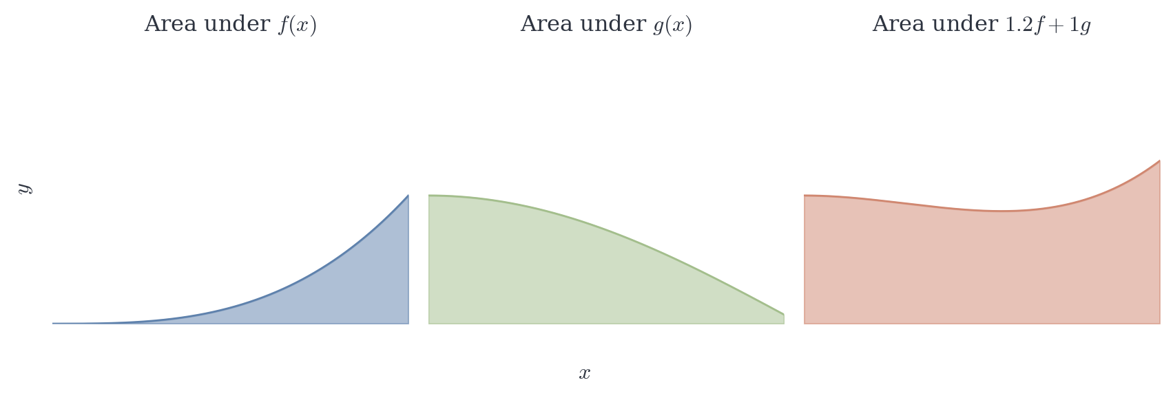
The integral, viewed as a map I : \mathscr{R}([a,b]) \to \mathbb{R} defined by I(f) = \int_a^b f, is a linear functional. It assigns a real number to each integrable function. Like the differential df_a, which was a linear functional on displacement vectors, the integral is a linear functional on function space.

Theorem 8.4 (Linearity) If f, g \in \mathscr{R}([a,b]) and \alpha, \beta \in \mathbb{R}, then \alpha f + \beta g \in \mathscr{R}([a,b]) and \int_a^b (\alpha f + \beta g) = \alpha \int_a^b f + \beta \int_a^b g.

Proof.

We make the observation: on any subinterval, \inf(\alpha f + \beta g) \geq \alpha \inf f + \beta \inf g and \sup(\alpha f + \beta g) \leq \alpha \sup f + \beta \sup g when \alpha, \beta \geq 0 (with appropriate adjustments for negative coefficients).

Given \varepsilon > 0, choose partitions P_1, P_2 such that U(f, P_1) - L(f, P_1) < \frac{\varepsilon}{2|\alpha|}, \quad U(g, P_2) - L(g, P_2) < \frac{\varepsilon}{2|\beta|}.

Let P = P_1 \cup P_2. Then P refines both, so U(f,P) - L(f,P) < \frac{\varepsilon}{2|\alpha|}, \quad U(g,P) - L(g,P) < \frac{\varepsilon}{2|\beta|}.

For \alpha f + \beta g, we have \begin{align*} U(\alpha f + \beta g, P) - L(\alpha f + \beta g, P) &\leq |\alpha|(U(f,P) - L(f,P)) + |\beta|(U(g,P) - L(g,P))\\ &< \varepsilon. \end{align*}

Thus \alpha f + \beta g \in \mathscr{R}([a,b]). The value follows by taking limits of upper and lower sums. \square

Beyond linearity, integrals preserve order. If one function lies below another pointwise, their integrals respect this ordering. This seemingly obvious fact requires proof—we must verify that the limit process (taking suprema and infima over all partitions) preserves inequalities.

Theorem 8.5 (Order Preservation) If f, g \in \mathscr{R}([a,b]) and f(x) \leq g(x) for all x \in [a,b], then \int_a^b f \leq \int_a^b g.

Proof.

The inequality f \leq g implies m_i(f) \leq m_i(g) and M_i(f) \leq M_i(g) on each subinterval. Thus L(f,P) \leq L(g,P) and U(f,P) \leq U(g,P) for every partition P. Taking suprema and infima preserves the inequality. \square

Corollary 8.1 If m \leq f(x) \leq M for all x \in [a,b], then m(b-a) \leq \int_a^b f \leq M(b-a).

This corollary provides immediate bounds on integrals when we know the range of the function—a useful tool for estimation.

Another fundamental property concerns how integrals behave when we split the interval of integration. Geometrically, the area under a curve from a to b should equal the area from a to c plus the area from c to b. But again, this requires proof—we’re working with limits of sums, and additivity must be verified carefully.

Theorem 8.6 (Additivity Over Intervals) If f \in \mathscr{R}([a,b]) and a < c < b, then f \in \mathscr{R}([a,c]), f \in \mathscr{R}([c,b]), and \int_a^b f = \int_a^c f + \int_c^b f.

Proof.

Any partition P of [a,b] that includes c decomposes into partitions P_1 of [a,c] and P_2 of [c,b]. Upper and lower sums satisfy L(f,P) = L(f,P_1) + L(f,P_2), \quad U(f,P) = U(f,P_1) + U(f,P_2).

Given \varepsilon > 0, choose P with U(f,P) - L(f,P) < \varepsilon. Refine to include c if necessary. Then [U(f,P_1) - L(f,P_1)] + [U(f,P_2) - L(f,P_2)] < \varepsilon.

Both gaps are nonnegative, so each is less than \varepsilon. Thus f \in \mathscr{R}([a,c]) and f \in \mathscr{R}([c,b]). Additivity of the integral follows from additivity of sums. \square

Having established linearity, order preservation, and additivity, we turn to products. This is less obvious than the previous properties—there’s no simple formula for the integral of a product in terms of the integrals of the factors (unlike sums). Nevertheless, the product of integrable functions is integrable, and the proof shows this.

Theorem 8.7 (Products of Integrable Functions) If f, g \in \mathscr{R}([a,b]), then fg \in \mathscr{R}([a,b]).

Proof.

We first show that if f \in \mathscr{R}([a,b]), then f^2 \in \mathscr{R}([a,b]).

Since f is integrable, it is bounded: there exists M > 0 such that |f(x)| \leq M for all x \in [a,b].

Given \varepsilon > 0, choose partition P such that U(f, P) - L(f, P) < \frac{\varepsilon}{2M}.

On each subinterval [x_{i-1}, x_i], let m_i = \inf\{f(x) : x \in [x_{i-1}, x_i]\}, \quad M_i = \sup\{f(x) : x \in [x_{i-1}, x_i]\}.

For f^2, observe that on [x_{i-1}, x_i], \sup\{f^2(x)\} - \inf\{f^2(x)\} \leq (M_i + |m_i|)(M_i - m_i) \leq 2M(M_i - m_i).

This uses the identity a^2 - b^2 = (a+b)(a-b) and the bound |f| \leq M.

Therefore, \begin{align*} U(f^2, P) - L(f^2, P) &= \sum_{i=1}^{n} [\sup f^2 - \inf f^2](x_i - x_{i-1}) \\ &\leq \sum_{i=1}^{n} 2M(M_i - m_i)(x_i - x_{i-1}) \\ &= 2M[U(f,P) - L(f,P)] \\ &< 2M \cdot \frac{\varepsilon}{2M} = \varepsilon. \end{align*}

Thus f^2 \in \mathscr{R}([a,b]).

Now, for the product fg, use the identity fg = \frac{1}{4}[(f+g)^2 - (f-g)^2].

Since f, g \in \mathscr{R}([a,b]), by linearity (Theorem 8.4), we have f+g \in \mathscr{R}([a,b]) and f-g \in \mathscr{R}([a,b]). By the result above, (f+g)^2 \in \mathscr{R}([a,b]) and (f-g)^2 \in \mathscr{R}([a,b]). By linearity again, fg = \frac{1}{4}[(f+g)^2 - (f-g)^2] \in \mathscr{R}([a,b]). \quad \square

The proof technique deserves comment. Rather than working directly with fg, we reduce to showing that f^2 is integrable, then use the algebraic identity to express fg in terms of squares. This is a common strategy in analysis: transform a difficult problem into a solved one via algebraic manipulation.

A particularly important special case concerns absolute values. The function |f| measures the magnitude of f without regard to sign. Geometrically, \int_a^b |f| gives the total area between the curve and the x-axis, counting both regions above and below the axis positively. This differs from \int_a^b f, which accounts for signed area (regions below the axis contribute negatively).

Theorem 8.8 (Integrability of |f|) If f \in \mathscr{R}([a,b]), then |f| \in \mathscr{R}([a,b]) and \left|\int_a^b f\right| \leq \int_a^b |f|.

Proof.

First, given \varepsilon > 0, choose partition P such that U(f, P) - L(f, P) < \varepsilon.

On each subinterval [x_{i-1}, x_i], let m_i = \inf\{f(x) : x \in [x_{i-1}, x_i]\}, \quad M_i = \sup\{f(x) : x \in [x_{i-1}, x_i]\}.

For any s, t \in [x_{i-1}, x_i], we have ||f(s)| - |f(t)|| \leq |f(s) - f(t)| \leq M_i - m_i.

This follows from the reverse triangle inequality: for any real numbers a, b, ||a| - |b|| \leq |a - b|.

Therefore, for |f| on [x_{i-1}, x_i], \sup|f| - \inf|f| \leq M_i - m_i.

Consequently, \begin{align*} U(|f|, P) - L(|f|, P) &= \sum_{i=1}^{n} [\sup|f| - \inf|f|](x_i - x_{i-1}) \\ &\leq \sum_{i=1}^{n} (M_i - m_i)(x_i - x_{i-1}) \\ &= U(f, P) - L(f, P) \\ &< \varepsilon. \end{align*}

Thus |f| \in \mathscr{R}([a,b]).

Next, since -|f(x)| \leq f(x) \leq |f(x)| for all x \in [a,b], by order preservation (Theorem 8.5), -\int_a^b |f| \leq \int_a^b f \leq \int_a^b |f|.

This is equivalent to \left|\int_a^b f\right| \leq \int_a^b |f|. \quad \square

8.10 Which Functions Are Integrable?

Not every bounded function is Riemann integrable. The canonical counterexample:

Dirichlet’s function: f(x) = \begin{cases} 1 & \text{if } x \in \mathbb{Q}, \\ 0 & \text{if } x \notin \mathbb{Q}. \end{cases}

On any subinterval [x_{i-1}, x_i], both rationals and irrationals are dense. Thus \inf f = 0 and \sup f = 1 on every subinterval. For any partition P, L(f,P) = 0, \quad U(f,P) = b-a.

The gap never shrinks. The function is not integrable.

This pathology arises from excessive discontinuity—the function jumps between 0 and 1 at every point. Continuous functions, by contrast, cannot oscillate so wildly. If f is continuous at a point, nearby values are close, which limits the difference between supremum and infimum on sufficiently small intervals. This intuition, made rigorous through uniform continuity, yields a fundamental positive result.

Before stating it, we need to establish that continuous functions on closed bounded intervals are uniformly continuous—a theorem of independent interest.

Uniform Continuity

The proof of Theorem 8.9 requires uniform continuity, which we state precisely:

Theorem (Uniform Continuity on Closed Intervals) If f : [a,b] \to \mathbb{R} is continuous, then for every \varepsilon > 0, there exists \delta > 0 such that for all x, y \in [a,b], |x - y| < \delta \implies |f(x) - f(y)| < \varepsilon.

Proof. Suppose, for contradiction, that f is not uniformly continuous. Then there exists \varepsilon_0 > 0 such that for every \delta > 0, we can find x, y \in [a,b] with |x-y| < \delta but |f(x) - f(y)| \geq \varepsilon_0.

Taking \delta = 1/n for n = 1, 2, 3, \ldots, we obtain sequences \{x_n\} and \{y_n\} in [a,b] such that |x_n - y_n| < \frac{1}{n} \quad \text{and} \quad |f(x_n) - f(y_n)| \geq \varepsilon_0.

Since [a,b] is closed and bounded, the Bolzano–Weierstrass theorem provides a convergent subsequence \{x_{n_k}\} with x_{n_k} \to p for some p \in [a,b].

Since |x_{n_k} - y_{n_k}| < 1/n_k \to 0, we also have y_{n_k} \to p.

By continuity of f at p, f(x_{n_k}) \to f(p) \quad \text{and} \quad f(y_{n_k}) \to f(p).

Therefore, |f(x_{n_k}) - f(y_{n_k})| \to 0, contradicting |f(x_{n_k}) - f(y_{n_k})| \geq \varepsilon_0 for all k. \square

The distinction between pointwise continuity and uniform continuity is crucial. Pointwise continuity says: for each x, there exists \delta (depending on both \varepsilon and x) such that nearby points map to nearby values. Uniform continuity strengthens this: there exists \delta (depending only on \varepsilon, not on x) that works simultaneously for all points in the domain.

On closed bounded intervals, the distinction collapses—continuity implies uniform continuity. This is a compactness argument: the function cannot oscillate arbitrarily rapidly because there’s nowhere for the oscillation to “escape to” at the boundaries.

With uniform continuity established, we can prove the main positive result about integrability.

Theorem 8.9 (Continuous Functions Are Integrable) If f : [a,b] \to \mathbb{R} is continuous, then f \in \mathscr{R}([a,b]).

Proof.

Continuous functions on closed bounded intervals are uniformly continuous (Uniform Continuity on Closed Intervals). Given \varepsilon > 0, there exists \delta > 0 such that |f(x) - f(y)| < \varepsilon/(b-a) whenever |x-y| < \delta.

Choose partition P with \|P\| < \delta. On each subinterval [x_{i-1}, x_i] of length less than \delta, the values of f vary by at most \varepsilon/(b-a). Thus M_i - m_i < \frac{\varepsilon}{b-a}.

Therefore, \begin{align*} U(f,P) - L(f,P) & = \sum_{i=1}^{n} (M_i - m_i)(x_i - x_{i-1}) \\ & < \frac{\varepsilon}{b-a} \sum_{i=1}^{n} (x_i - x_{i-1}) \\ &= \frac{\varepsilon}{b-a} \cdot (b-a) \\ &= \varepsilon. \end{align*}

And we’re done. \square

The proof shows precisely how uniform continuity controls the gap between upper and lower sums. By choosing partitions with sufficiently small mesh, we can make M_i - m_i uniformly small across all subintervals, which directly translates to making U(f,P) - L(f,P) small.

Beyond continuous functions, another natural class admits integration: monotone functions. A function that consistently increases (or decreases) cannot oscillate wildly—it crosses each horizontal line at most once. This structural constraint ensures integrability.

Theorem 8.10 (Monotone Functions Are Integrable) If f : [a,b] \to \mathbb{R} is monotone, then f \in \mathscr{R}([a,b]).

Proof.

Assume f is increasing (the decreasing case is similar). On each subinterval [x_{i-1}, x_i], we have m_i = f(x_{i-1}), \quad M_i = f(x_i).

Thus U(f,P) - L(f,P) = \sum_{i=1}^{n} [f(x_i) - f(x_{i-1})](x_i - x_{i-1}).

For an equal partition with \Delta x = (b-a)/n, \begin{align*} U(f,P) - L(f,P) &= \Delta x \sum_{i=1}^{n} [f(x_i) - f(x_{i-1})]\\ & = \Delta x [f(b) - f(a)] \\ &= \frac{(b-a)[f(b) - f(a)]}{n}. \end{align*}

As n \to \infty, this approaches 0. \square

The telescoping sum in the proof is characteristic of monotone function arguments—the total variation f(b) - f(a) is distributed across n subintervals, and as n grows, each piece becomes negligible when multiplied by \Delta x = (b-a)/n.

Functions with finitely many discontinuities are also integrable, though we omit the proof. The intuition is that discontinuities contribute zero to the integral (they occur at isolated points, which have zero “length”), so as long as there are finitely many, they don’t disrupt the limiting process. For our purposes, continuous and piecewise continuous functions suffice.

8.11 The Integral as a Linear Functional

We close by emphasizing structure. The integral defines a map I : \mathscr{R}([a,b]) \to \mathbb{R}, \quad I(f) = \int_a^b f(x) \, dx.

This map is linear (Theorem 8.4): I(\alpha f + \beta g) = \alpha I(f) + \beta I(g). The integral is a functional—it assigns a real number to each function in its domain.

Compare to the differential df_a, which was a linear functional on displacement space. The differential measured “how much f changes along displacement h.” The integral measures “how much f accumulates over [a,b].”

Differentiation	Integration
Local (at a point)	Global (over an interval)
Extracts instantaneous rate	Accumulates total change
Linear map: D(f+g) = Df + Dg	Linear functional: \int (f+g) = \int f + \int g
Sensitive to small perturbations	Robust to changes at isolated points

This duality—local versus global, instantaneous versus cumulative—is the organizing principle of calculus. Differentiation and integration are inverse operations in a precise sense. The Fundamental Theorem of Calculus, which we develop next, makes this duality explicit: the integral of a derivative recovers total change, and differentiation inverts the accumulation process.