7 Taylor Series
7.1 Polynomial Approximation
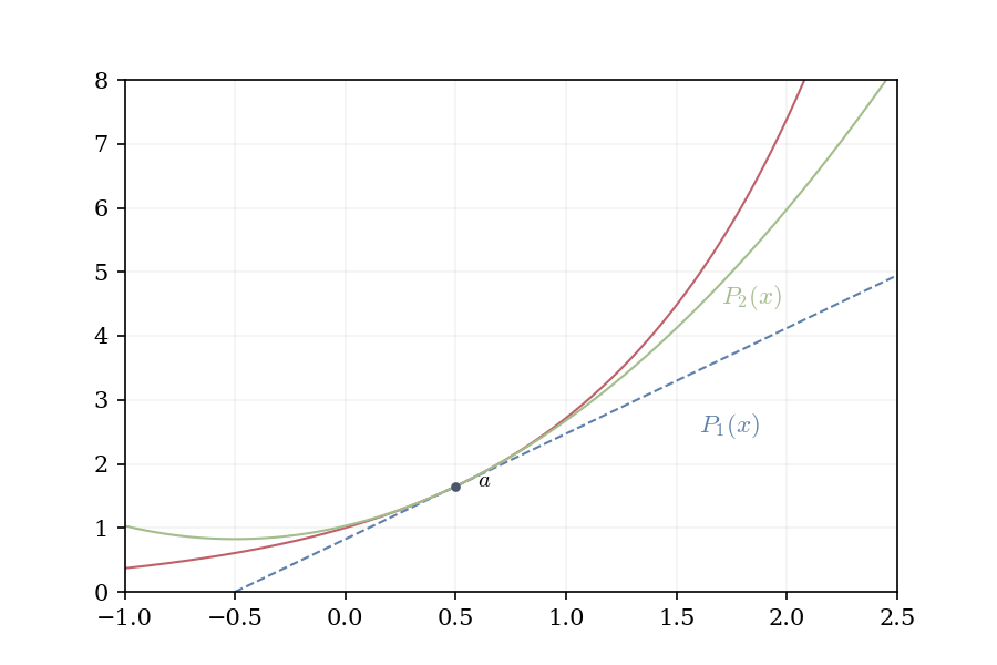
We built differential calculus on a single idea: near any point, a smooth function (recall smoothness classes: C^\infty, infinitely differentiable) looks linear. The tangent line L(x) = f(a) + f'(a)(x-a) captures this local linearity. The differential df_a(h) = f'(a)h measures approximate change near a.
The linearity holds only in a neighborhood of a. As we move away from a, the approximation deteriorates. For f(x) = e^x at a = 0, the linear approximation 1 + x yields f(1) \approx 2, whereas the actual value is e \approx 2.718, representing a significant error.
We seek a better approximation.
If f is twice differentiable, additional information is available: f'(a) provides the instantaneous rate of change, and f''(a) indicates whether this rate is increasing or decreasing. This reflects the curvature. A parabolic approximation should outperform the linear one.
The natural candidate is: P(x) = f(a) + f'(a)(x-a) + \frac{f''(a)}{2}(x-a)^2
Why the factor \frac{1}{2}? Differentiating twice yields: P'(x) = f'(a) + f''(a)(x-a), \quad P''(x) = f''(a).
At x = a: P(a) = f(a), P'(a) = f'(a), P''(a) = f''(a). The parabola matches f and its first two derivatives at a. The factor \frac{1}{2} ensures that P''(a) = f''(a), rather than 2f''(a).
If functions that are twice differentiable are locally parabolic, consider thrice-differentiable functions. We add a cubic term: Q(x) = f(a) + f'(a)(x-a) + \frac{f''(a)}{2}(x-a)^2 + \frac{f'''(a)}{6}(x-a)^3
Differentiating confirms that Q^{(k)}(a) = f^{(k)}(a) for k = 0, 1, 2, 3. The pattern is evident: to match the nth derivative, the coefficient must be \frac{f^{(n)}(a)}{n!}.
7.2 Polynomial Spaces
Recall from Section 6.1 that polynomials of degree at most n form a vector space—we can add them and scale them by constants. A convenient basis for this space (when approximating near x = a) is \{1, (x-a), (x-a)^2, (x-a)^3, \ldots, (x-a)^n\}.
These functions are linearly independent: no nontrivial linear combination produces the zero polynomial. Every polynomial P of degree \leq n can be written uniquely as P(x) = c_0 \cdot 1 + c_1 (x-a) + c_2 (x-a)^2 + \cdots + c_n (x-a)^n.
The coefficients c_0, c_1, \ldots, c_n are the coordinates of P in this basis. This is the same structure we studied in § Vectors and Linear Maps: a finite-dimensional vector space with a basis adapted to the point a.
Why choose this basis? Because (x-a)^k vanishes at x = a when k \geq 1, facilitating the matching of function values and derivatives there. The basis is adapted to differentiation at a.
Given f, we seek the best polynomial approximation of degree \leq n. That is, we want coefficients c_0, c_1, \ldots, c_n such that P(x) = \sum_{k=0}^{n} c_k (x-a)^k approximates f near a.
What constitutes the “best approximation”? We require that P matches f and its first n derivatives at a: P(a) = f(a), \quad P'(a) = f'(a), \quad P''(a) = f''(a), \quad \ldots, \quad P^{(n)}(a) = f^{(n)}(a).
This is the most information we can extract from f at the single point a—the function value and all its derivatives up to order n.
7.3 Derivatives and Coefficients
We now examine how the derivatives determine the coefficients.
Start with P(x) = c_0 + c_1(x-a) + c_2(x-a)^2 + c_3(x-a)^3 + \cdots + c_n(x-a)^n.
Evaluate at x = a: P(a) = c_0.
So c_0 = f(a). The zeroth coefficient equals the function value.
Differentiate once: P'(x) = c_1 + 2c_2(x-a) + 3c_3(x-a)^2 + \cdots + nc_n(x-a)^{n-1}.
Evaluate at x = a: P'(a) = c_1.
So c_1 = f'(a). The first coefficient equals the first derivative.
Differentiate again: P''(x) = 2c_2 + 6c_3(x-a) + 12c_4(x-a)^2 + \cdots
Evaluate at x = a: P''(a) = 2c_2.
So c_2 = \frac{f''(a)}{2}. The second coefficient equals half the second derivative.
The pattern is as follows: each differentiation isolates one coefficient, introducing a factorial factor. The kth derivative of (x-a)^k equals k! at x = a, whereas the kth derivative of (x-a)^j for j < k vanishes, and for j > k still contains terms with (x-a) that vanish at a.
Computing the kth derivative: P^{(k)}(x) = k! c_k + \text{(terms containing $(x-a)$)}.
Evaluating at x = a: P^{(k)}(a) = k! c_k.
Therefore: c_k = \frac{f^{(k)}(a)}{k!}.
The derivatives at a determine the coordinates in the basis \{1, (x-a), (x-a)^2, \ldots\}.
7.4 The Normalized Basis
The standard basis \{1, x, x^2, x^3, \ldots\} for \mathcal{P}_n is natural but not unique. Any linearly independent spanning set of n+1 polynomials forms a basis. For studying Taylor series, a different basis proves more convenient.
Definition 7.1 (Normalized Basis) The normalized basis for \mathcal{P}_n is \mathcal{B}_{\text{norm}} = \left\{1, x, \frac{x^2}{2!}, \frac{x^3}{3!}, \ldots, \frac{x^n}{n!}\right\}.
This basis differs from the standard basis only by scaling: the k-th element is x^k / k! instead of x^k. The factors 1/k! have a special property when we examine derivatives.
Coordinates in the normalized basis: A polynomial written as p(x) = b_0 \cdot 1 + b_1 \cdot x + b_2 \cdot \frac{x^2}{2!} + b_3 \cdot \frac{x^3}{3!} + \cdots + b_n \cdot \frac{x^n}{n!} has coordinate vector (b_0, b_1, b_2, \ldots, b_n).
Evaluating p and its derivatives at x = 0 gives: p(0) = b_0, \quad p'(0) = b_1, \quad p''(0) = b_2, \quad p'''(0) = b_3, \quad \ldots, \quad p^{(k)}(0) = b_k.
The coordinates are exactly the derivatives at x = 0.
This property makes the normalized basis natural for Taylor series. A function f with derivatives f^{(k)}(a) at a point a has Taylor series \sum_{k=0}^{\infty} f^{(k)}(a) \cdot \frac{(x-a)^k}{k!}.
This is the infinite linear combination with coordinates (f(a), f'(a), f''(a), \ldots) in the normalized basis centered at a. The factorial factors in the basis elements absorb the factorial in the derivative formula, leaving the coordinates as pure derivatives.
Definition 7.2 (Taylor Polynomial) Let f be n times differentiable at a. The nth Taylor polynomial is T_n(x) = \sum_{k=0}^{n} \frac{f^{(k)}(a)}{k!}(x-a)^k.
This is the unique polynomial of degree \leq n that matches f and its first n derivatives at a.
Taylor polynomials are linear combinations of basis functions (x-a)^k, with weights \frac{f^{(k)}(a)}{k!} determined by derivatives. The function f projects onto the space of degree-n polynomials, and its coordinates in the standard basis \{(x-a)^k\} are the scaled derivatives.
The factor \frac{1}{k!} is not arbitrary—it comes from the basis choice.
Consider the basis \{1, (x-a), (x-a)^2, (x-a)^3, \ldots\}. When we differentiate (x-a)^k exactly k times, we get k!. This means the kth derivative at a “sees” the coefficient c_k multiplied by k!.
To make the coordinate system work cleanly—so that the kth coordinate directly encodes information about the kth derivative—we normalize by k!.
Think of it as a change of basis. The “raw” basis \{1, (x-a), (x-a)^2, \ldots\} is convenient algebraically, but the normalized basis \left\{1, (x-a), \frac{(x-a)^2}{2!}, \frac{(x-a)^3}{3!}, \ldots, \frac{(x-a)^n}{n!}\right\} is adapted to differentiation. In this basis, the coordinates are simply f^{(k)}(a)—no factorials needed.
Writing the Taylor polynomial in the normalized basis: T_n(x) = f(a) \cdot 1 + f'(a) \cdot (x-a) + f''(a) \cdot \frac{(x-a)^2}{2!} + \cdots + f^{(n)}(a) \cdot \frac{(x-a)^n}{n!}.
Each coefficient is now directly the derivative. The basis functions absorb the factorial.
The second derivative d^2f is a bilinear form (the Hessian matrix), and 1/2! ensures the quadratic approximation respects this bilinearity.
In quantum mechanics and functional analysis, similar normalizations appear when working with orthogonal polynomial bases (Hermite, Laguerre polynomials). The factorial ensures that inner products and operator actions remain well-behaved.
7.5 Taylor Series
As n increases, the Taylor polynomial T_n matches more and more derivatives of f at a. Each additional term in the basis expansion captures higher-order behavior.
Consider the limit as n tends to infinity.
If the sequence T_0(x), T_1(x), T_2(x), \ldots converges to f(x), we obtain an infinite linear combination: f(x) = \sum_{k=0}^{\infty} \frac{f^{(k)}(a)}{k!}(x-a)^k.
This is the Taylor series—a power series with coefficients determined by derivatives at a. The function f is completely reconstructed from its behavior at the single point a.
Definition 7.3 (Taylor Series) Let f \in C^\infty (infinitely differentiable) at a. The Taylor series of f centered at a is \sum_{n=0}^{\infty} \frac{f^{(n)}(a)}{n!}(x-a)^n.
When a = 0, this is the Maclaurin series.
In the power series chapter, we established that if f(x) = \sum c_n x^n converges on some interval, then the coefficients must be c_n = \frac{f^{(n)}(0)}{n!} (uniqueness of power series). Taylor series make this construction explicit: given a smooth function (C^\infty), build its power series from derivatives.
The Taylor series always exists if f \in C^\infty. But it may not converge. Even if it converges, it may not converge to f.
The coordinates \frac{f^{(k)}(a)}{k!} are well-defined, but the infinite linear combination \sum_{k=0}^{\infty} \frac{f^{(k)}(a)}{k!}(x-a)^k is a series that may or may not have a finite sum. And even if it does, that sum might differ from f(x).
To determine convergence, we must control the approximation error.
7.6 Taylor’s Remainder
The nth Taylor polynomial gives an approximation. Define the remainder: R_n(x) = f(x) - T_n(x).
In the linear algebra language: R_n(x) is the projection error—the part of f that lies outside the span of \{1, (x-a), \ldots, (x-a)^n\}.
For the Taylor series to converge to f(x), we need R_n(x) \to 0 as n \to \infty. As we add more basis functions, the projection error must vanish.
But how do we estimate R_n(x) without already knowing f(x)?
The key is that R_n(x) can be expressed using the (n+1)st derivative at an intermediate point.
Theorem 7.1 (Taylor’s Theorem (Lagrange Remainder)) Let f be (n+1) times differentiable on an interval containing a and x. Then there exists c strictly between a and x such that R_n(x) = \frac{f^{(n+1)}(c)}{(n+1)!}(x-a)^{n+1}.
The remainder has the form of the next basis term (x-a)^{n+1}, weighted by the derivative f^{(n+1)}(c) evaluated at some intermediate point c.
If we continued the Taylor expansion to degree n+1, we would add the term \frac{f^{(n+1)}(a)}{(n+1)!}(x-a)^{n+1}.
The actual error R_n(x) has this same form, but uses f^{(n+1)}(c) instead of f^{(n+1)}(a). The error resembles the next term in the expansion, evaluated at a shifted point.
This is a generalization of the Mean Value Theorem: just as f(x) - f(a) = f'(c)(x-a) for some c, the higher-order error R_n(x) equals the next-order term evaluated at an intermediate point.
Define the auxiliary function \phi(t) = f(x) - \sum_{k=0}^{n} \frac{f^{(k)}(t)}{k!}(x-t)^k - K(x-t)^{n+1} where K is chosen so that \phi(a) = 0. This forces K = \frac{f(x) - T_n(x)}{(x-a)^{n+1}} = \frac{R_n(x)}{(x-a)^{n+1}}.
By construction, \phi(x) = 0 (all terms vanish when t = x). Since \phi(a) = \phi(x) = 0 and \phi is differentiable, Rolle’s theorem provides c between a and x where \phi'(c) = 0.
Differentiating \phi term-by-term (most terms telescope by the product rule): \phi'(t) = -\frac{f^{(n+1)}(t)}{n!}(x-t)^n + K(n+1)(x-t)^n.
Setting \phi'(c) = 0 and solving: K = \frac{f^{(n+1)}(c)}{(n+1)!}.
Therefore R_n(x) = \frac{f^{(n+1)}(c)}{(n+1)!}(x-a)^{n+1}. \quad \square
7.7 Convergence of Taylor Series
Taylor’s theorem gives an explicit formula for R_n(x). Convergence reduces to showing this remainder vanishes.
Corollary 7.1 (Error Bound) If |f^{(n+1)}(t)| \leq M for all t between a and x, then |R_n(x)| \leq \frac{M}{(n+1)!}|x-a|^{n+1}.
To prove the Taylor series converges to f(x):
Bound |f^{(n+1)}(t)| by some M (possibly depending on x)
Show \frac{M|x-a|^{n+1}}{(n+1)!} \to 0 as n \to \infty
Conclude R_n(x) \to 0, so the infinite linear combination converges to f(x)
Example 7.1 (Taylor Series of e^x Converges Everywhere) For f(x) = e^x, every derivative equals e^x. On [0, x] with x > 0, we have f^{(n+1)}(t) = e^t \leq e^x. Thus |R_n(x)| \leq \frac{e^x \cdot x^{n+1}}{(n+1)!}.
For fixed x, from the power series chapter we know (by the ratio test) that \sum \frac{x^n}{n!} converges, so \frac{x^{n+1}}{(n+1)!} \to 0. Therefore R_n(x) \to 0.
Conclusion: e^x = \sum_{n=0}^{\infty} \frac{x^n}{n!} = \sum_{n=0}^{\infty} f^{(n)}(0) \cdot \frac{x^n}{n!}.
The function e^x equals its infinite linear combination in the basis \{x^n/n!\}, with coordinates given by derivatives at 0. The radius of convergence is R = \infty.
[Animation: Show error |R_n(x)| as a function of x for increasing n, watching it shrink to zero uniformly on any bounded interval]
7.7.0.1 Other Common Taylor Series
The sine function. For f(x) = \sin(x) at a = 0, the derivatives cycle with period 4. At x = 0 f^{(0)}(0) = 0, \quad f^{(1)}(0) = 1, \quad f^{(2)}(0) = 0, \quad f^{(3)}(0) = -1, \quad f^{(4)}(0) = 0, \quad \ldots
Only odd derivatives are nonzero, alternating in sign \sin(x) = \sum_{n=0}^{\infty} \frac{(-1)^n x^{2n+1}}{(2n+1)!} = x - \frac{x^3}{3!} + \frac{x^5}{5!} - \frac{x^7}{7!} + \cdots
All derivatives of \sin are bounded by 1, so |R_n(x)| \leq \frac{|x|^{n+1}}{(n+1)!} \to 0 for all x. The radius of convergence is R = \infty.
The cosine function. For f(x) = \cos(x) at a = 0, we note that \cos x = \frac{d}{dx}\left(\sin x\right), hence \begin{align*} \cos x &= \frac{d}{dx}\left(\sum_{n=0}^{\infty} \frac{(-1)^n x^{2n+1}}{(2n+1)!}\right) \\ &= \sum_{n=0}^{\infty} \frac{(-1)^n}{(2n+1)!}\,\frac{d}{dx}\left(x^{2n+1}\right)\\ &= \sum_{n=0}^{\infty} \frac{(-1)^n x^{2n}}{(2n)!}= 1 - \frac{x^2}{2!} + \frac{x^4}{4!} - \frac{x^6}{6!} + \cdots \end{align*}
With radius of convergence, R = \infty.
Example 7.2 (The Geometric Series) For f(x) = \frac{1}{1-x} at a = 0, compute derivatives f(x) = (1-x)^{-1}, \quad f'(x) = (1-x)^{-2}, \quad f''(x) = 2(1-x)^{-3}, \quad f'''(x) = 6(1-x)^{-4}, \quad \ldots
In general, f^{(n)}(x) = n!(1-x)^{-(n+1)}, so f^{(n)}(0) = n!.
The Taylor series is \frac{1}{1-x} = \sum_{n=0}^{\infty} \frac{n!}{n!} x^n = \sum_{n=0}^{\infty} x^n.
This recovers the geometric series. The radius of convergence is R = 1 (ratio test).
For |x| < 1, the remainder satisfies R_n(x) = \frac{f^{(n+1)}(c)}{(n+1)!}x^{n+1} = \frac{x^{n+1}}{1-c} for some c between 0 and x. Since |c| < |x| < 1, we have \frac{1}{1-c} < \frac{1}{1-|x|}, bounded. Thus |R_n(x)| \to 0 as n \to \infty.
For |x| \geq 1, the series diverges (geometric series divergence).
7.8 Limitations of Taylor Series
Does every C^\infty function admit a Taylor series representation?
No. Consider the following example: f(x) = \begin{cases} e^{-1/x^2} & x \neq 0 \\ 0 & x = 0 \end{cases}
This is C^\infty everywhere. At x = 0, repeated L’Hôpital’s rule shows f^{(n)}(0) = 0 for all n.
The Taylor series at 0: \sum_{n=0}^{\infty} \frac{0}{n!} x^n = 0.
But f(x) \neq 0 for x \neq 0. The series converges, but to the incorrect function.
What is the cause of this failure? The coordinates \{f^{(n)}(0)\} are all zero. In the basis \{x^n/n!\}, the function f has coordinate vector (0, 0, 0, \ldots). The projection onto the span of polynomial basis functions is the zero function.
Yet f is not the zero function. It lies outside the span of \{x^n/n!\}—the space of polynomials (even allowing infinitely many terms) is not large enough to represent all C^\infty functions.
Geometric picture: We’re trying to express f as a linear combination of basis functions. If f is not in the span of those basis functions, the expansion fails. The Taylor series gives the best polynomial approximation in a precise sense (matching derivatives), but that approximation might not equal f.
For most functions (e^x, \sin x, \cos x, rational functions on appropriate domains), the span of \{(x-a)^n\} is large enough. The Taylor series converges to the function. However, this is not always the case.
7.9 Power and Taylor Series
The power series chapter asked: given coefficients c_n, when does \sum c_n x^n converge, and what function does it define?
This chapter answers the inverse question: given a function f, can we find coefficients such that f(x) = \sum c_n x^n?
The Taylor series provides the answer: if f \in C^\infty and its Taylor series converges to f, then the coefficients are uniquely determined: c_n = \frac{f^{(n)}(a)}{n!}.
Two perspectives on the same object:
- Power series perspective: Start with coefficients, build a function via infinite sum, determine radius of convergence
- Taylor series perspective: Start with a function, extract coefficients from derivatives, check whether the series converges back to the function
Both frameworks are essential:
- Power series theory tells us where convergence is possible (radius R, interval of convergence)
- Taylor series theory tells us which functions have power series representations (those where R_n(x) \to 0)
Together, they reveal that C^\infty functions with controlled derivatives can be represented exactly as infinite polynomials—and those representations inherit all the nice properties of polynomials: continuity, differentiability, algebraic manipulability.
7.10 Properties of Taylor Series
Taylor series are coordinate representations of functions in the basis \{1, (x-a), (x-a)^2, \ldots\}, with coordinates determined by derivatives: f(x) = \sum_{k=0}^{\infty} \underbrace{\frac{f^{(k)}(a)}{k!}}_{\text{coordinate}} \cdot \underbrace{(x-a)^k}_{\text{basis function}}.
The factorial normalization ensures that derivatives determine coordinates directly. The basis \{(x-a)^k/k!\} is adapted to differentiation.
Convergence depends on whether the projection error R_n(x) vanishes as n \to \infty. This reduces to bounding derivatives via Taylor’s theorem.
Higher-order differentials d^kf_a provide the functional perspective: the k-th coordinate encodes the k-th order behavior of f at a.
When the Taylor series converges to f, the function is completely determined by its derivatives at a single point—all information about f is encoded in the sequence \{f^{(n)}(a)\}_{n=0}^{\infty}.
A noteworthy consequence is that evaluating f and all its derivatives at one location allows reconstruction of f everywhere within the radius of convergence. The Taylor series is the explicit reconstruction formula, built from the differential structure we developed in Calculus 1.