3 The Cauchy Criterion
3.1 General Principles
In the previous chapter, we established the definition of series convergence: \sum a_n converges if its partial sums s_n = \sum_{k=1}^{n} a_k converge to a limit. This reduction from infinite sums to sequence limits proved immediately fruitful. For geometric series and telescoping series, we computed s_n explicitly and determined convergence by evaluating \lim_{n \to \infty} s_n.
But consider the series \sum_{n=1}^{\infty} \frac{1}{n^2}, \quad \sum_{n=1}^{\infty} \frac{1}{n!}, \quad \sum_{n=1}^{\infty} \frac{\sin(n)}{n^2}.
For these, no simple closed form for s_n exists. The partial sums grow in complicated ways, and computing their limits directly is impossible. Yet we wish to determine whether these series converge. How can we analyze convergence when we cannot compute partial sums?
This chapter establishes two foundational tools. First, we prove that series behave well under algebraic operations and that convergence depends only on tail behavior—the behavior far out in the sequence. Second, we develop the Cauchy criterion, a method for testing convergence without requiring knowledge of the limit. This criterion will prove to be the theoretical foundation for all the convergence tests we develop in subsequent chapters.
3.2 Linearity of Series
Since series reduce to sequences, and sequences obey limit laws, series inherit algebraic structure automatically. The proof amounts to observing that partial sums respect addition and scalar multiplication.
Theorem 3.1 (Linearity of Series) If \sum a_n = A and \sum b_n = B, then \sum (a_n + b_n) = A + B and \sum ca_n = cA for any c \in \mathbb{R}.
Proof.
Let s_n = \sum_{k=1}^{n} a_k and t_n = \sum_{k=1}^{n} b_k. By hypothesis, s_n \to A and t_n \to B.
For the sum, observe that the nth partial sum of \sum (a_n + b_n) is \sum_{k=1}^{n} (a_k + b_k) = \sum_{k=1}^{n} a_k + \sum_{k=1}^{n} b_k = s_n + t_n.
By the sum rule for sequence limits, \lim_{n \to \infty} (s_n + t_n) = A + B.
For scalar multiplication, the nth partial sum of \sum ca_n is \sum_{k=1}^{n} ca_k = c\sum_{k=1}^{n} a_k = cs_n.
By the constant multiple rule for sequence limits, \lim_{n \to \infty} cs_n = cA. \square
These properties mirror the linearity of the limit operator itself. Addition and scalar multiplication commute with taking limits—the limit of a sum is the sum of limits, and the limit of a constant multiple is the constant multiple of the limit. Series inherit this structure because they are defined through limits.
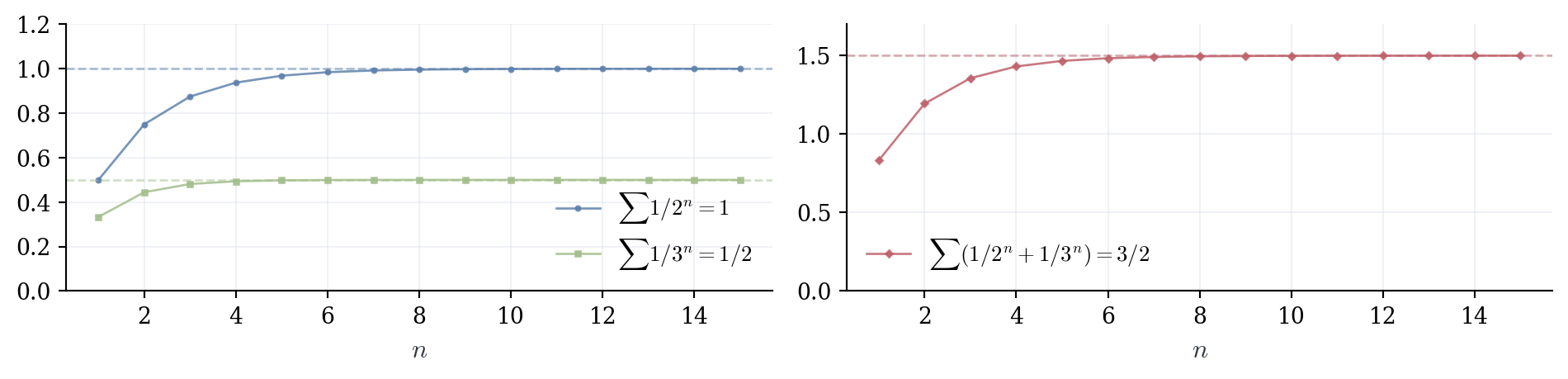
Linearity allows us to decompose complicated series into simpler pieces, analyze each separately, and combine results. Consider \sum_{n=1}^{\infty} \left(\frac{1}{2^n} + \frac{1}{3^n}\right). Both pieces are geometric with |r| < 1, giving \sum_{n=1}^{\infty} \frac{1}{2^n} = 1 and \sum_{n=1}^{\infty} \frac{1}{3^n} = \frac{1}{2}. By linearity, the combined series equals 1 + \frac{1}{2} = \frac{3}{2}.
Similarly, the series \sum_{n=1}^{\infty} \frac{5}{2^n} factors as 5 \sum_{n=1}^{\infty} \frac{1}{2^n} = 5 \cdot 1 = 5.
Warning. Products behave differently. In general, \sum a_n b_n \neq \left(\sum a_n\right)\left(\sum b_n\right). The product of two series requires a more sophisticated treatment involving rearrangement. Multiplication is not term-by-term.
3.3 Tail Behavior
As we’ve seen, convergence is about behavior “at infinity,” not about any finite collection of terms. We encountered this first in the definition of sequence convergence—the initial terms a_1, a_2, \ldots, a_{N-1} are irrelevant. Only what happens beyond some threshold N matters.
The same principle governs series. Changing finitely many terms alters the partial sums by a constant shift, but does not affect whether the sequence of partial sums converges. This observation has important practical consequences.
Theorem 3.2 (Finite Changes Do Not Affect Convergence) Let N \in \mathbb{N}. The series \sum_{n=1}^{\infty} a_n converges if and only if \sum_{n=N}^{\infty} a_n converges.
When both converge, \sum_{n=1}^{\infty} a_n = \underbrace{\sum_{n=1}^{N-1} a_n}_{\text{finite}} + \sum_{n=N}^{\infty} a_n.
Proof.
Let s_n = \sum_{k=1}^{n} a_k denote the partial sums of the original series, and let t_n = \sum_{k=N}^{n} a_k for n \geq N denote the partial sums starting from index N.
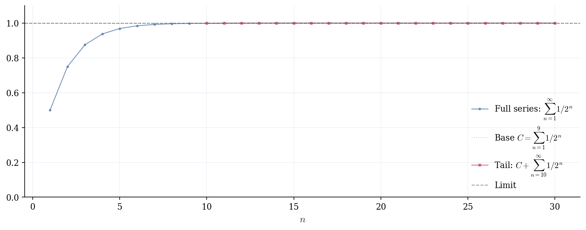
Define the constant C = \sum_{k=1}^{N-1} a_k, which is a finite sum, hence a well-defined real number. For n \geq N, s_n = \sum_{k=1}^{n} a_k = \sum_{k=1}^{N-1} a_k + \sum_{k=N}^{n} a_k = C + t_n.
The sequences \{s_n\} and \{t_n\} differ by the constant C. Since adding a constant to every term does not affect whether a sequence converges, s_n converges if and only if t_n converges.
When both converge, \lim_{n \to \infty} s_n = C + \lim_{n \to \infty} t_n. \square
Consequence. Adding, removing, or changing finitely many terms does not affect whether a series converges. The value of the sum may change, but convergence or divergence is determined entirely by the tail.
This theorem justifies a practical strategy: when testing convergence, we may ignore the first million terms, start indexing wherever convenient, and focus entirely on the behavior as n \to \infty. The initial terms contribute a finite constant to the sum, but they cannot determine whether the infinite process converges.
The series \sum_{n=5}^{\infty} \frac{1}{2^n} differs from \sum_{n=0}^{\infty} \frac{1}{2^n} = 2 only in the first four terms. Computing directly, we get 2 - \left(1 + \frac{1}{2} + \frac{1}{4} + \frac{1}{8} + \frac{1}{16}\right) = \frac{1}{16}. Alternatively, recognize this as geometric with first term a = 1/32 and ratio r = 1/2, giving \frac{1/32}{1-1/2} = \frac{1}{16}.
When testing whether \sum_{n=1}^{\infty} \frac{1}{n^2} converges, the first few terms—1, \frac{1}{4}, \frac{1}{9}, \frac{1}{16}—tell us nothing definitive. We could equally well test \sum_{n=1000}^{\infty} \frac{1}{n^2}. The convergence question concerns behavior as n \to \infty, not the values at any particular finite stage.
3.4 Cauchy Sequences
We have successfully analyzed geometric and telescoping series by computing their partial sums s_n explicitly. But this direct approach fails for most series. Consider again \sum_{n=1}^{\infty} \frac{1}{n^2}. The partial sums s_n = 1 + \frac{1}{4} + \frac{1}{9} + \cdots + \frac{1}{n^2} have no simple closed form. We cannot compute \lim_{n \to \infty} s_n directly. Yet the series converges (to \pi^2/6, though this is far from obvious), and we need a method to verify convergence without knowing or computing the limit.
From the discussion above, one may realize that we do not actually need to know the limit. The definition of convergence requires only that s_n approaches some real number, not that we can identify what that number is. If we can verify that the sequence \{s_n\} has the properties characteristic of convergent sequences—without reference to any particular limit—we will have established convergence.
This is where the Cauchy criterion enters. It provides an alternative characterization of convergence that makes no mention of the limit value.
3.5 Cauchy Sequences
Let us return to a fundamental question from differential calculus: what does it mean for a sequence to converge? The standard definition says that \{\vartheta_n\} converges if there exists L \in \mathbb{R} such that \vartheta_n approaches L. But this definition has a logical structure that can be awkward in practice: it requires us to know or guess the limit L before we can verify convergence.
Consider testing whether \vartheta_n = \sum_{k=1}^{n} \frac{1}{k^2} converges. The standard definition asks: is there an L such that |\vartheta_n - L| becomes arbitrarily small? But we do not know L. How can we verify that \vartheta_n approaches a number we cannot identify?
There is another way to think about convergence, one that focuses on the sequence itself rather than on some external limit point. If \vartheta_n approaches some limit L, then as n increases, the terms \vartheta_n must get closer and closer to L. But if \vartheta_m is close to L and \vartheta_n is close to L, then \vartheta_m and \vartheta_n must be close to each other.
More precisely, suppose \vartheta_n \to L. Given \varepsilon > 0, we can find N such that for all n \geq N, the term \vartheta_n lies within \varepsilon/2 of L. Then for any two indices m, n \geq N, both \vartheta_m and \vartheta_n lie within \varepsilon/2 of L, which means they lie within \varepsilon of each other by the triangle inequality |\vartheta_m - \vartheta_n| \leq |\vartheta_m - L| + |L - \vartheta_n| < \frac{\varepsilon}{2} + \frac{\varepsilon}{2} = \varepsilon.
This reasoning suggests a property that convergent sequences must possess: eventually, all terms become arbitrarily close to one another. This property characterizes convergence completely—it is both necessary and sufficient.
The advantage of this perspective is that it makes no reference to the limit L. We test whether terms cluster together, not whether they approach any particular value. For sequences whose limits we cannot compute, this reformulation is invaluable.
Definition 3.1 (Cauchy Sequence) A sequence \{\vartheta_n\} is Cauchy if for every \varepsilon > 0, there exists N \in \mathbb{N} such that |\vartheta_n - \vartheta_m| < \varepsilon \quad \text{for all } n, m \geq N.
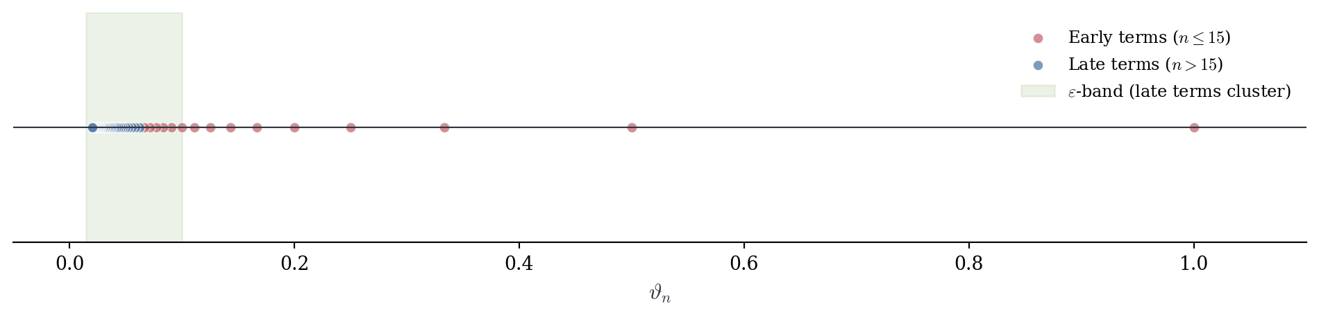
The condition requires that all pairs of terms beyond the threshold N lie within \varepsilon of each other. The sequence is “clustering”—the terms are not just approaching something, they are approaching each other.
Imagine plotting the terms \vartheta_1, \vartheta_2, \vartheta_3, \ldots on the real line. A Cauchy sequence is one where, if you go far enough out (choose N large enough), all subsequent terms lie in an interval of width at most \varepsilon. They have stopped wandering—they are confined to an arbitrarily small region, even though we may not know where that region is located on the line.
The sequence \vartheta_n = 1/n provides a simple example. Given \varepsilon > 0, we must find N such that |\vartheta_m - \vartheta_n| < \varepsilon whenever m, n \geq N. Assuming m \geq n, we have
|\vartheta_m - \vartheta_n| = \frac{1}{n} - \frac{1}{m} \leq \frac{1}{n}.
To ensure 1/n < \varepsilon, choose N > 1/\varepsilon. Then for all n \geq N, we get
|\vartheta_m - \vartheta_n| \leq \frac{1}{n} \leq \frac{1}{N} < \varepsilon.
The sequence is Cauchy. Notice that we verified this without mentioning that \vartheta_n \to 0—the Cauchy property stands on its own.
By contrast, the sequence \vartheta_n = (-1)^n is not Cauchy. Take \varepsilon = 1. For any N, we can choose n even and m odd with both n, m \geq N. Then
|\vartheta_m - \vartheta_n| = |(-1) - 1| = 2 > \varepsilon.
No matter how far out we go, terms continue to differ by 2. They never cluster together.
Consider now the sequence defined by partial sums, \vartheta_n = \sum_{k=1}^{n} \frac{1}{k^2}. We do not know that \vartheta_n \to \pi^2/6. Can we verify the Cauchy property directly? For m > n, the difference is
|\vartheta_m - \vartheta_n| = \sum_{k=n+1}^{m} \frac{1}{k^2}.
We bound this tail sum. For k \geq 2, observe that \frac{1}{k^2} < \frac{1}{k(k-1)}, since
\frac{1}{k(k-1)} - \frac{1}{k^2} = \frac{1}{k^2(k-1)} > 0.
Therefore,
\sum_{k=n+1}^{m} \frac{1}{k^2} < \sum_{k=n+1}^{m} \frac{1}{k(k-1)}.
The right side is telescoping. And,
\frac{1}{k(k-1)} = \frac{1}{k-1} - \frac{1}{k},
so the sum equals \frac{1}{n} - \frac{1}{m} < \frac{1}{n}. Thus |\vartheta_m - \vartheta_n| < \frac{1}{n}. Given \varepsilon > 0, choose N > \frac{1}{\varepsilon}. Then for all m > n \geq N, we have
|\vartheta_m - \vartheta_n| < \frac{1}{n} \leq \frac{1}{N} < \varepsilon.
The sequence is Cauchy. We have verified this without computing \vartheta_n explicitly and without knowing the limit. The clustering property alone suffices.
3.5.1 An Equivalence
We have seen that convergent sequences are Cauchy—if \vartheta_n \to L, then terms eventually cluster around L, hence around each other. The triangle inequality makes this rigorous.
Theorem 3.3 (Convergent Sequences are Cauchy) If \{\vartheta_n\} converges, then \{\vartheta_n\} is Cauchy.
Proof.
Suppose \vartheta_n \to L. Given \varepsilon > 0, there exists N such that |\vartheta_n - L| < \varepsilon/2 for all n \geq N.
For m, n \geq N, the triangle inequality gives |\vartheta_m - \vartheta_n| = |\vartheta_m - L + L - \vartheta_n| \leq |\vartheta_m - L| + |L - \vartheta_n| < \frac{\varepsilon}{2} + \frac{\varepsilon}{2} = \varepsilon. \quad \square
The converse is deeper. Does every Cauchy sequence converge? Intuitively, if terms cluster together in a smaller and smaller region, that region must be collapsing onto some point—but where is that point? For the sequence to converge, the limit must exist as a real number. The fact that this is always true is a fundamental property of \mathbb{R}.
Theorem 3.4 (Cauchy Sequences Converge (Completeness of \mathbb{R})) Every Cauchy sequence in \mathbb{R} converges to some L \in \mathbb{R}.
Proof sketch.
We outline the argument, leaving some technical details to a course in real analysis.
First, Cauchy sequences are bounded. Take \varepsilon = 1. There exists N such that |\vartheta_n - \vartheta_m| < 1 for all n, m \geq N. In particular, for all n \geq N, we have |\vartheta_n| \leq |\vartheta_n - \vartheta_n| + |\vartheta_n| < 1 + |\vartheta_n|. Define M = \max(|\vartheta_1|, |\vartheta_2|, \ldots, |\vartheta_{N-1}|, |\vartheta_n| + 1). Then |\vartheta_n| \leq M for all n. The sequence is bounded.
By the Bolzano–Weierstrass theorem (analysis), every bounded sequence has a convergent subsequence. Let \{\vartheta_{n_k}\} be a subsequence with \vartheta_{n_k} \to L for some L \in \mathbb{R}.
We show that the Cauchy property forces \vartheta_n \to L for the entire sequence, not just the subsequence. Given \varepsilon > 0, the Cauchy property provides N_1 such that |\vartheta_n - \vartheta_m| < \varepsilon/2 for all n, m \geq N_1. Convergence of the subsequence provides K such that |\vartheta_{n_k} - L| < \varepsilon/2 for all k \geq K. Choose k large enough that both n_k \geq N_1 and k \geq K. Then for any n \geq N_1, we have |\vartheta_n - L| \leq |\vartheta_n - \vartheta_{n_k}| + |\vartheta_{n_k} - L| < \frac{\varepsilon}{2} + \frac{\varepsilon}{2} = \varepsilon. Thus \vartheta_n \to L. \square
This theorem is not really about sequences—it is about the real numbers. The statement “every Cauchy sequence converges” is called completeness, and it is precisely what distinguishes \mathbb{R} from \mathbb{Q}. In the rational numbers, Cauchy sequences need not converge. Consider the decimal approximations to \sqrt{2}, the sequence 1, 1.4, 1.41, 1.414, 1.4142, \ldots is Cauchy when viewed as rational numbers—the terms cluster together. But the limit \sqrt{2} is irrational. The sequence has no limit within \mathbb{Q}. The rationals have “gaps,” and Cauchy sequences can fall into these gaps. The real numbers have no such gaps. Every Cauchy sequence converges to a real number. This property—completeness—is what allows calculus to function. Without it, limits might not exist, series might not converge even when they should, and the foundations would collapse.
Combining both directions:
Corollary 3.1 (Cauchy Criterion for Sequences) A sequence \{\vartheta_n\} in \mathbb{R} converges if and only if it is Cauchy.
This equivalence is powerful: to test convergence, we need not know the limit. We verify only that terms eventually cluster together. For sequences whose limits we cannot compute—which includes most sequences arising in practice—this reformulation is indispensable.
3.6 Cauchy Criterion
Now we translate the Cauchy characterization from sequences to series. A series \sum a_n converges if and only if its partial sums s_n = \sum_{k=1}^{n} a_k form a convergent sequence. By the Cauchy criterion, this occurs if and only if \{s_n\} is Cauchy.
What does it mean for partial sums to be Cauchy? Consider two partial sums s_m and s_n with m > n. Their difference is s_m - s_n = \sum_{k=1}^{m} a_k - \sum_{k=1}^{n} a_k = \sum_{k=n+1}^{m} a_k.
This is a tail sum—the sum of consecutive terms from a_{n+1} through a_m. The Cauchy property for \{s_n\} becomes a statement about how small these tail sums can be made.
Theorem 3.5 (Cauchy Criterion for Series) The series \sum_{n=1}^{\infty} a_n converges if and only if for every \varepsilon > 0, there exists N \in \mathbb{N} such that \left|\sum_{k=n+1}^{m} a_k\right| < \varepsilon \quad \text{for all } m > n \geq N.
Proof.
The series converges if and only if the sequence of partial sums \{s_n\} converges. By the Cauchy criterion for sequences, this occurs if and only if \{s_n\} is Cauchy. The sequence \{s_n\} is Cauchy if and only if for every \varepsilon > 0, there exists N such that |s_m - s_n| < \varepsilon for all m > n \geq N. Since s_m - s_n = \sum_{k=n+1}^{m} a_k, the result follows immediately. \square
The Cauchy criterion says: a series converges if and only if tail sums can be made arbitrarily small. Once we go far enough out (beyond index N), any finite chunk of terms from a_{n+1} to a_m contributes less than \varepsilon to the total.
This reformulation has two important advantages: it isolates tail behavior (generalizing the divergence test Section 3.8), and it requires no knowledge of the limit. We need not compute s_n explicitly or know what value the series converges to. We verify only that tail sums become small—an estimate, not a calculation.
3.7 Applications
We prove that \sum_{n=1}^{\infty} \frac{1}{n^2} converges without knowing the sum. For m > n, we bound the tail sum. As shown earlier, for k \geq 2, we have \frac{1}{k^2} < \frac{1}{k(k-1)} = \frac{1}{k-1} - \frac{1}{k}. Therefore, \sum_{k=n+1}^{m} \frac{1}{k^2} < \sum_{k=n+1}^{m} \left(\frac{1}{k-1} - \frac{1}{k}\right) = \frac{1}{n} - \frac{1}{m} < \frac{1}{n}.
Given \varepsilon > 0, choose N > \frac{1}{\varepsilon}. Then for all m > n \geq N, we have \left|\sum_{k=n+1}^{m} \frac{1}{k^2}\right| < \frac{1}{n} \leq \frac{1}{N} < \varepsilon. By the Cauchy criterion, the series converges. We proved convergence without computing any partial sum and without knowing the limit. The proof works entirely by estimating tail sums.
The harmonic series \sum_{n=1}^{\infty} \frac{1}{n} diverges (see the grouping argument in the introduction). The Cauchy criterion provides an alternative perspective on this divergence: for the tail from a_{n+1} to a_{2n}, we have \sum_{k=n+1}^{2n} \frac{1}{k} \geq n \cdot \frac{1}{2n} = \frac{1}{2}, since each of the n terms satisfies \frac{1}{k} \geq \frac{1}{2n}. Thus tail sums remain bounded below by 1/2, regardless of how large n becomes. The Cauchy criterion fails because tail sums do not shrink to zero.
For geometric series with a_n = ar^{n-1} and |r| < 1, the tail sum satisfies \sum_{k=n+1}^{m} ar^{k-1} = ar^n \sum_{j=0}^{m-n-1} r^j = ar^n \frac{1-r^{m-n}}{1-r}.
Since |r|^{m-n} \leq 1 when |r| < 1, we have \left|\frac{1-r^{m-n}}{1-r}\right| \leq \frac{2}{|1-r|}. Therefore, \left|\sum_{k=n+1}^{m} ar^{k-1}\right| \leq \frac{2|a|}{|1-r|} |r|^n. Since |r| < 1, we have |r|^n \to 0. Given \varepsilon > 0, choose N such that \frac{2|a|}{|1-r|} |r|^N < \varepsilon. Then for m > n \geq N, the tail bound holds, confirming convergence without computing s_n = a\frac{1-r^n}{1-r} explicitly.
3.8 Divergence Test
The Cauchy criterion has a simple but important consequence. If \sum a_n converges, the Cauchy criterion holds. Given \varepsilon > 0, there exists N such that \left|\sum_{k=n+1}^{m} a_k\right| < \varepsilon for all m > n \geq N. Taking m = n+1 gives |a_{n+1}| < \varepsilon for all n \geq N. Thus a_n \to 0.
Corollary 3.2 (Necessary Condition for Convergence) If \sum a_n converges, then \lim_{n \to \infty} a_n = 0.
This recovers the divergence test from the previous chapter. The Cauchy criterion provides a unified framework: the divergence test is the special case m = n+1.
The series \sum_{n=1}^{\infty} \frac{n}{n+1} has terms a_n = \frac{n}{n+1} \to 1 \neq 0. By the divergence test, the series diverges. Similarly, \sum_{n=1}^{\infty} \cos(n) diverges since its terms oscillate and do not approach zero.
Recall that the converse fails: a_n \to 0 is necessary but not sufficient for convergence. The harmonic series provides the canonical counterexample.